Writing Genetic Algorithms in Rust!

Intro

Hi everyone! Today, we’ll talk about an interesting class of algorithms known as Genetic Algorithms. We will then implement a Rust library that acts as a wrapper around training Genetic Algorithms, and lets users train them after implementing a trait. Then, we will use the library to solve the following problems, 2 of which are very hard (NP-hard) problems:

1. Finding the maximum of a two-variable real function
2. The Traveling Salesman Problem
3. The Knapsack Problem

Without further ado, let’s get started!

Genetic Algorithms

As their name suggests, Genetic Algorithms (or GAs for short), are algorithms inspired by the biological concepts of Genetics and Evolution. The first computer simulation of evolution was created in 1954 by Nils Aall Barricelli, a Mathematician. They were then expanded upon by Australian quantitative geneticist Alex Fraser in 1957. Most GAs involve the optimization (constrained or unconstrained, as we’ll see today) of some cost/loss function. For example, GAs can be used to find the minimum of a function, or the shortest Hamiltonian cycle in a Graph (if you don’t know what that means, don’t worry, we’ll cover it later :)). The vast majority of Genetic Algorithms work as follows:

1. Initialize a population of possible solutions, called chromosomes randomly: for example, if we’re trying to maximize a real function of two variables x and y where 0<=x<=10 and 0<=y<=10, each chromosome in our population is a random point in the aforementioned region.
   This can be likened to populating a natural habitat, such as a rainforest, with a type of animal, such as an elephant, where each animal has different genes, although all animals are of the same type. For example, we can have one elephant with larger ears and one elephant with smaller ears
2. Evaluate a fitness function F for each chromosome that tells us how good the chromosome is as a solution to our problem. For example, in the case of maximizing a real function, the fitness function is simply the function we are trying to maximize. This is named after the concept of fitness in biology, which describes the reproductive success of an organism
3. Using the values of the fitness function, make a probability distribution, sometimes called the selection distribution, that tells us the probability of reproduction for each chromosome. For example, we can define the selection probability of a chromosome c to be the fitness of c divided by the sum of all fitnesses. Note that the more fit a chromosome is, the higher we want its probability of mating to be, so that its good attributes can pass onto the next generation. This mimics the process of natural selection: organisms that are more adapted to their environments have a larger chance of surviving and making offspring
4. Using the selection distribution, pick pairs of chromosomes from the current generation with replacement, meaning that one chromosome may reproduce more than once. Each such pair of chromosomes is then passed through an operation called a crossover, which generates two new offspring which share the properties of their parents, similar to biological reproduction
5. Finally, we apply, with a certain (typically low) probability, a mutation operation. This operation introduces noise into the training process of the algorithm, and can help it escape local optima. Mutation can come in many forms: for example, in a problem where the chromosomes are bit string, mutation can be flipping a random bit with a certain probability
6. Steps 4 and 5 are repeated until we generate the entire new generation, typically with the same size of the original generation That’s it! This process is then repeated for a certain number of iterations, and then the most fit chromosome (either in the last generation or throughout all generations) is picked. To implement this in Rust, I first created a trait called Chromosome which lets the algorithm evolve structures:

// How to treat the structure as a chromosome? i.e. how should it reproduce
// and how likely is it to be selected for reproduction
pub trait Chromosome
where
Self: Sized,
{
	// How should two chromosomes of this type be crossed together to produce two new offspring?
	fn crossover(x: Self, y: Self) -> (Self, Self);
	// Create a new random chromosome
	fn random() -> Self;
	// How fit is this chromosome?
	fn fitness(&self) -> f64;
	// How should this chromosome mutate?
	fn mutate(&self, mutations: &[bool]) -> Self;
}

Then, I made a structure called Run, which stores the hyperparameters of the algorithm, along with other data such as the current generation:

// A run of a genetic algorithm
pub struct Run<T: Chromosome> {
	// How many generations do we want this algorithm to go on for?
	num_iter: usize,
	// What is the probability of mutation (i.e. randomly bit flipping after a crossover)?
	p_mutation: f64,
	// Do we want to always keep the fitter part of the population?
	// are kept and all of the next generation is generated through natural selection & reproduction
	n_keep: usize,
	// What is the population size?
	n_pop: usize,
	// How many parameters does each chromosome have? For example, 2D points have two parameters: x and y
	n_params: usize,
	// How do we select which chromosomes are likely to reproduce?
	selection: Selection,
	// The current generation
	gen: Vec<T>,
	// Best-so-far vector of the optimal values of the cost function along with the chromosomes
	// that yielded them
	best_so_far: Vec<(T, f64)>,
}

The n_keep parameter is useful when implementing the selection process, because some algorithms want to always keep the upper part of the population (e.g. the upper half of chromosomes with the highest fitness) in the next generation and then make them reproduce amongst themselves, with probabilities proportional to their place. When we want to use other selection types we simply set it to 0 to indicate that none of the chromosomes in the current generation should directly pass on to the next generation. The Selection enum is defined as follows, and contains 3 types of selection processes:

// Types of ways to generate the probability distribution that controls
// which chromosomes are more likely to reproduce
pub enum Selection {
	// Fitness of the current chromosome / Sum of fitnesses
	Fraction,
	// Only keep the upper N_KEEP items of the population and let them reproduce
	// with probabilities proportional to their place (i.e. first place is most likely to reproduce)
	UpperItems,
	// Softmax function (exp'd fitness / sum of exp'd fitnesses)
	Softmax,
}

The meat of the Run struct is in a method called begin, which implements the evolution process and repeats it for the specified number of iterations:

// Run the algorithm for the specified number of iterations
// If 'verbose' is set to true, the entire history of the fittest chromosome
// in each generation along with its value is returned
// Otherwise, only the fittest one in the last generation
pub fn begin(&mut self) -> Vec<(T, f64)> {
	// Initialize the first generation by generating N_pop random chromosomes
	for _ in 0..self.n_pop {
		self.gen.push(T::random());
	}
	// Used later for sampling random chromosomes
	let mut rng = thread_rng();
	let uni = Uniform::new(0f64, 1f64);
	let mut_dist = Bernoulli::new(self.p_mutation).unwrap();
	
	for _ in 0..self.num_iter {
		// Sort the chromosomes in the current generation by fitness
		let mut chromo_by_fit: Vec<(&T, f64)> =
		self.gen.iter().map(|c| (c, c.fitness())).collect();
		chromo_by_fit.sort_by(|a, b| a.1.total_cmp(&b.1));
		// Put them in descending order
		chromo_by_fit.reverse();
		// Push the fittest chromosome in the current generation to the best_so_far vector
		let best = chromo_by_fit.first().unwrap();
		self.best_so_far.push((best.0.clone(), best.1));
		// Generate the new generation:
		// 1. Take the fittest N_keep chromosomes in the current generation and add them
		// 2. Generate the rest through natural selection
		let mut next_gen = vec![];
		// Step 1 - The fittest N_keep chromosomes are the last N_keep in chromo_by_fit
		for (c, _) in &chromo_by_fit[0..self.n_keep] {
			next_gen.push((*c).clone());
		}
		// Step 2 - The rest of the chromosomes are generated through natural selection
		for _ in 0..(self.n_pop - self.n_keep) / 2 {
			let parent1 = self
			.random_parent(uni, &mut rng, &chromo_by_fit)
			.expect("Cannot sample a random parent from an empty population!");
			let parent2 = self
			.random_parent(uni, &mut rng, &chromo_by_fit)
			.expect("Cannot sample a random parent from an empty population!");
			// Perform a crossover
			let (child1, child2) = T::crossover(parent1, parent2);
			// Introduce mutations randomly
			let mutations: Vec<bool> = mut_dist.sample_iter(&mut rng).take(self.n_params).collect();
			let child1 = child1.mutate(mutations.as_slice());
			let child2 = child2.mutate(mutations.as_slice());
			// Push to the next generation
			next_gen.push(child1);
			next_gen.push(child2);
		}
		// Assign it to the next gen
		self.gen = next_gen;
	}
	
	self.best_so_far.clone()
}

The function starts by initializing the first generation using a method called random, which is implemented in the Chromosome trait. This function initializes a new structure with random attributes. Then, it repeats the evolution process for the desired number of iterations:

1. It computes the fitness for each chromosome in the current generation and then sorts them by fitness (in decreasing order)
2. It pushes the best chromosome in the current generation to the best_so_far vector, which shows the history of the run
3. It then starts to make the next generation using the following two steps:
4. Passing the N_keep fittest chromosomes in the current generation directly on to the next generation
5. Sampling random parents according to the selection distribution, and crossing them over (N_pop - N_keep) / 2 times. We divide by 2 since each crossover produces 2 offspring
6. Applying mutations to the 2 offspring using the mutate method defined in the trait. This method takes in a vector of randomly generated bools the size of the number of parameters (e.g. for a 2D point we have 2 parameters), and then mutates the offspring in some way defined by the user Finally, the random_parent function samples a random parent using the selection distribution as follows:

// Sample a random chromosome from this generation WRT the selection distribution
// This is done by sampling a random number from 0 to 1 from a uniform distribution
// and then picking the chromosome corresponding to that interval
// for example, if we have P(C1) = 0.5 P(C2) = 0.25 and P(C3) = 0.25
// If the random number y is smaller than 0.5, we pick C1
// If it's between 0.5 and 0.5 + 0.25 = 0.75, we pick C2
// and if it's larger than 0.75, we pick C3
fn random_parent(
&self,
dist: Uniform<f64>,
rng: &mut ThreadRng,
chromo_by_fit: &Vec<(&T, f64)>,
) -> Option<T> {
	// The chromosomes by probability to be reproduced
	// We call enumerate to also pass the place of each element by fitness
	let mut chromo_by_prob: Vec<(&T, f64)> = chromo_by_fit
	.iter()
	.enumerate()
	.map(|(i, (a, _))| (*a, match self.selection {
		// Different ways to compute the selection probability
		Selection::Fraction => {
			let fit_sum = chromo_by_fit.iter().map(|(_, fit)| fit).sum::<f64>();
			a.fitness() / fit_sum
		},
		Selection::UpperItems => {
			let place = i + 1;
			if 1 <= place && place <= self.n_keep {
				(self.n_keep as f64 - place as f64 + 1f64)
				/ ((1..self.n_keep + 1).sum::<usize>() as f64)
			} else {
				0f64
			}
		}
		Selection::Softmax => {
			let fit_exp_sum = chromo_by_fit.iter().map(|(_, fit)| fit.exp()).sum::<f64>();
			a.fitness().exp() / fit_exp_sum
		}
	}))
	.collect();
	
	chromo_by_prob.sort_by(|a, b| a.1.total_cmp(&b.1));
	chromo_by_prob.reverse();
	// Generate a random number y
	let y = dist.sample(rng);
	let mut prev = 0f64;
	let mut curr = 0f64;
	
	for chromo in chromo_by_prob {
		curr += chromo.1;
		
		if prev <= y && y < curr {
			return Some(chromo.0.clone());
		}
		
		prev = curr;
	}
	
	None
}

It first generates the probability distribution from the fitnesses according to the type of selection selected by the user. Then, it samples a random chromosome from the distribution by first sorting the chromosomes by their probability of selection, so that each two probabilities create an interval, and then sampling a uniform number from (0, 1), and selecting a chromosome according to the intervals. For example, if we have selection probabilities of 0.5, 0.3, and 0.2, we have the following three intervals:

1. (0, 0.5)
2. (0.5 0.5+0.3) = (0.5, 0.8)
3. (0.8, 0.8 + 0.2) = (0.8, 1) If the random number we picked is in interval 1, we return chromosome 1. If it’s in the second interval, we return chromosome 2, and if it’s in the third interval, we return chromosome 3. We can see that chromosomes with larger probabilities have a larger chance to be selected, since their interval is larger. Now that we saw how GAs work, let’s look at some examples!

   Maximizing a Multivariate Function

   In our first example, we’ll tackle the problem of maximizing/minimizing (effectively it’s the same problem, since maximizing the negative of a function is equivalent to minimizing a function) a multivariate function within some bounded region. The function we’ll use is f(x, y) = 0.8 * sin(x) * cos(2y) - 3 * cos(x - y). Since our function takes in a point in 2D space, our chromosomes, which are possible solutions to the problem, are 2D points:

struct Point {
	x: f64,
	y: f64,
}

Now, we need to implement the Chromosome trait for this Point structure so that the library will know how to evolve it. The Chromosome trait looks as follows:

// How to treat the structure as a chromosome? i.e. how should it reproduce
// and how likely is it to be selected for reproduction
pub trait Chromosome
where
Self: Sized,
{
	// How should two chromosomes of this type be crossed together to produce two new offspring?
	fn crossover(x: Self, y: Self) -> (Self, Self);
	// Create a new random chromosome
	fn random() -> Self;
	// How fit is this chromosome?
	fn fitness(&self) -> f64;
	// How should this chromosome mutate?
	fn mutate(&self, mutations: &[bool]) -> Self;
}

So we need to implement these 4 operations. Let’s start with the easiest one: the fitness function is simply the function f(x, y) we want to maximize:

fn fitness(&self) -> f64 {
	// The function we want to maximize
	0.8 * self.x.sin() * (2f64 * self.y).cos() - 3f64 * (self.x - self.y).cos()
}

Now let’s write the next easiest function: generating a random point:

fn random() -> Self {
	let mut rng = thread_rng();
	let x = rng.gen_range(0f64..10f64);
	let y = rng.gen_range(0f64..10f64);
	
	Point { x, y }
}

Now we need to define the crossover operation. Given two points x and y, we can randomly swap one of their coordinates to create 2 offspring:

fn crossover(x: Self, y: Self) -> (Self, Self) {
	let mut rng = thread_rng();
	// Do we change x or y?
	let param = rng.gen_range(0..2);
	
	match param {
		// Swap x coordinate
		0 => {
			let child1 = Point {
				x: y.x,
				y: x.y,
			};
			let child2 = Point {
				x: x.x,
				y: y.y,
			};
			
			(child1, child2)
		}
		// Swap y coordinate
		1 => {
		let child1 = Point {
			x: x.x,
			y: y.y,
		};
		let child2 = Point {
			x: y.x,
			y: x.y,
		};
		
		(child1, child2)
		}
		// Shouldn't happen
		_ => {
		(x, y)
		}
	}
}

Finally, we need to implement the mutation operation. Remember that this operation gets a vector of bools that tell us which parameters have mutated. As a mutation, we will simply change each of the coordinates that mutated to a random number:

// Mutate each of the parameters of the chromosome
// as input, we get a vector of N_params booleans, true indicating that we should mutate a parameter
// and false indicating that we should keep it the same
fn mutate(&self, mutations: &[bool]) -> Self {
	let mut rng = thread_rng();
	
	// If a mutation happened, we replace the mutated coordinate with a random number from 0 to 10
	Point {
		x: if mutations[0] == true {
			rng.gen_range(0f64..10f64)
		} else {
			self.x
		},
		y: if mutations[1] == true {
			rng.gen_range(0f64..10f64)
		} else {
			self.y
		},
	}
}

Awesome! We’ve implemented all the items in the trait. Let’s run the GA now:

const N_KEEP: usize = 6;
const N_POP: usize = 12;

fn main() {
	let mut run = Run::<Point>::new(200, 0.2, N_KEEP, N_POP, 2, evolve::Selection::UpperItems);
	let history = run.begin();
	
	for i in 0..200 {
		println!("{}\t{}", history[i].0, history[i].1);
	}
}

In the final generation, we see that the most fit point and values are:

(4.713143183295525, 1.5697884689229724) 3.7999934899421293

To decide whether this is a good or bad solution, let’s try to find an upper bound the on the maximum of f(x, y) = 0.8 * sin(x) * cos(2y) - 3 * cos(x - y). Since the upper and lower bounds of the sine/cosine functions are 1 and -1, respectively (meaning for all x, -1 <= sin(x) <= 1), we have sin(x) <= 1, cos(2y) <= 1, and cos(x - y) >= -1. Therefore, f(x, y) = 0.8 * sin(x) * cos(2y) - 3 * cos(x - y) <= 0.8 * 1 * 1 - 3 * (-1) = 3.8. Our approximated maximum has a value of 3.7999934899421293, so this is really really close to the true upper bound! It has an error on the order of 1e-6. The algorithm actually converged earlier than the full 200 iterations, so we could have used early stopping to stop running it then. Nice! Now, let’s get onto the next problem, which is discrete, unlike this one.

The Traveling Salesman Problem

This is one of the most famous problems in computer science, and it involves optimization in graphs. If you are unfamiliar with graphs, they are essentially a data structure that shows relationships between objects. Each object is called a vertex, and between each two connected vertices we have an edge: 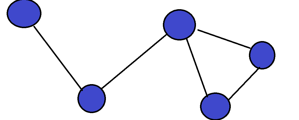Graphs are a very versatile data structure, and they can be used to represent a lot of things such as social networks or transportation networks. We can also put weights on edges/nodes, which shows us how “expensive” each edge/node is. For example, if we have a transportation network, we can let all of the cities be nodes, and all roads connecting two cities be edges. We can then weight each road according to its length. In the Traveling Salesman Problem (TSP for short), we are given such a weighted graph, which is also complete (there exists an edge between all pairs of vertices): 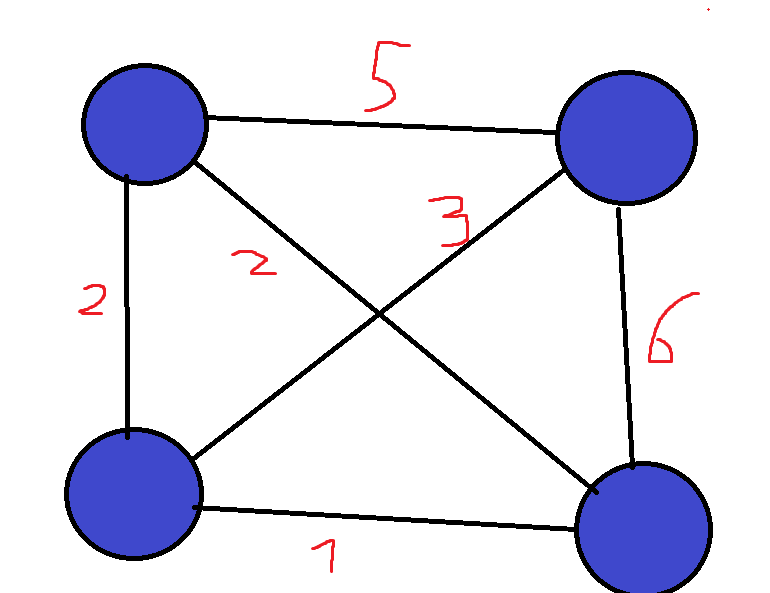Our goal is to find the cheapest way to start at one city, visit all cities, and then return to the city we started at. The total weight of a cycle is defined as the sum of the weights of its edges. Such a cycle that visits all nodes in the graph is called a Hamiltonian Cycle, named after William Rowan Hamilton, an Irish mathematician. For example, in the above graph, the green highlighted edges in the next figure are an example of a Hamiltonian cycle. Each node shows at which point in time we visit it: 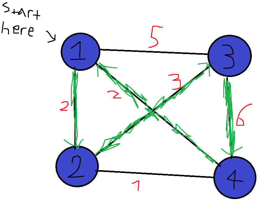The above cycle has a weight of 2 + 3 + 6 + 2 = 13. This problem may seem pretty simple, but there hasn’t been discovered an exact algorithm for it that runs in polynomial time yet! Now that we understand the problem, let’s write a GA for it using the library. Given a complete graph with N vertices, we can label each vertex with a unique number from 1 to N. Because the graph is complete, we can go from any node to any other node, so we can let our chromosomes be permutations of the integers from 1 to N, which show the order of visited nodes. For example, in the above 4-complete graph, we can represent the green cycle with the permutation 1,2,3,4. The cycle 3->2->1->4->3 can be represented as 3,2,1,4. In Rust, we define the chromosomes as follows:

struct Permutation {
	// Permutation of cities 1..n - the order of cities to visit
	perm: [usize; NUM_CITIES],
}

Then, we need to implement the Chromosome trait. Let’s start by generating a random Permutation, which simply amounts to shuffling the vector vec![1, ..., n]:

fn random() -> Self {
	let mut rng = thread_rng();
	// Create a random permutation
	let mut perm: Vec<usize> = (0..NUM_CITIES).collect();
	perm.shuffle(&mut rng);
	// Return the Permutation
	Permutation {
		perm: perm.try_into().unwrap(),
	}
}

Now, let’s define the fitness function. We define the fitness to be the cost of the cycle, which is the sum of all edge weights:

fn fitness(&self) -> f64 {
	let mut cost = 0f64;
	let dist_mat = DistMatrix::new();
	
	for i in 0..NUM_CITIES - 1 {
		let city_a = self.perm[i];
		let city_b = self.perm[i + 1];
		
		cost += dist_mat.dist(city_a, city_b);
	}
	
	// Getting from the last city to the first city
	cost += dist_mat.dist(self.perm[NUM_CITIES - 1], self.perm[0]);
	
	-1f64 * cost as f64
}

The last addition is because we also need to return from the last city to the first city. Because the graph is complete, we can represent the distances with a symmetric matrix, whose i,j-th entry is the edge cost between city i and city j. At the end, we multiply by -1 since we want to maximize the negative of the cost, which is equivalent to minimizing the cost. The DistMatrix struct helps us takes care of the weights, and loads the distance matrix between 20 random 2D points I generated with Python from a file. We treat each 2D point as a node, and the distances between them as edge costs. Now, let’s define the crossover operation. The operation here is more complex than before, because simply swapping a random index in the permutation can result in duplicates. For example, if we have the permutations 2, 1, 3, 4 and 4, 3, 1, 2, and we swap index 2, we’ll get 2, 3, 3, 4 and 4, 1, 1, 2, which contain duplicates and therefore are invalid permutations. Instead, we will start by swapping a random index, and then swap the duplicates until there are none left (Figure taken from “An Introduction to Genetic Algorithms” by Jenna Carr, Table 5): 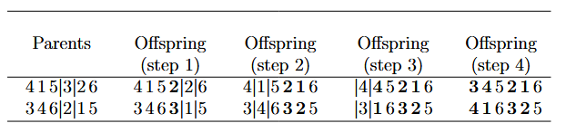We implement this in Rust as follows:

fn crossover(x: Self, y: Self) -> (Self, Self) {
	let mut first_offspring = x.perm;
	let mut second_offspring = y.perm;
	// Cycle crossover
	let mut rng = thread_rng();
	let mut visited = vec![];
	// Exchange a random index
	let random_idx = rng.gen_range(0..NUM_CITIES);
	let tmp = first_offspring[random_idx];
	// The current element which is a duplicate in the first offspring
	let mut dup_elem;
	first_offspring[random_idx] = second_offspring[random_idx];
	dup_elem = second_offspring[random_idx];
	second_offspring[random_idx] = tmp;
	
	visited.push(random_idx);
	
	loop {
		for i in 0..NUM_CITIES {
			// If this is the duplicate and we haven't touched it yet
			if first_offspring[i] == dup_elem && !visited.contains(&i) {
				let tmp = first_offspring[i];
				first_offspring[i] = second_offspring[i];
				dup_elem = second_offspring[i];
				second_offspring[i] = tmp;
				visited.push(i);
			}
		}
		
		// If there are no duplicates
		if first_offspring.iter().sum::<usize>() == (0..NUM_CITIES).sum() {
			break;
		}
	} 
	
	let first_offspring = Permutation {
	perm: first_offspring,
	};
	
	let second_offspring = Permutation {
	perm: second_offspring,
	};
	
	(first_offspring, second_offspring)
}

Finally, in the mutation operation, we simply swap two random indexes of the permutation, which keeps the permutation valid:

fn mutate(&self, mutations: &[bool]) -> Self {
	let is_mut = mutations[0];
	let mut rng = thread_rng();
	let perm = self.perm;
	
	if is_mut {
		let mut mutated_perm = perm;
		// Generate two random indexes
		let rand_idx_1 = rng.gen_range(0..NUM_CITIES);
		let rand_idx_2 = rng.gen_range(0..NUM_CITIES);
		// Swap between them
		let tmp = mutated_perm[rand_idx_1];
		mutated_perm[rand_idx_1] = mutated_perm[rand_idx_2];
		mutated_perm[rand_idx_2] = tmp;
		
		Permutation { perm: mutated_perm }
	} else {
		Permutation { perm }
	}
}

Great! Now, let’s run the algorithm:

const NUM_CITIES: usize = 20;
const N_POP: usize = 20;
const N_KEEP: usize = 10;

fn main() {
	let mut run =
	Run::<Permutation>::new(200, 0.2, N_KEEP, N_POP, 1, evolve::Selection::UpperItems);
	
	let history = run.begin();
	
	for (perm, fitness) in history {
		println!("{}\t{}", perm, fitness);
	}
}

Running it, we get the following output:

10 19 17 2 5 0 3 7 15 14 11 13 12 16 9 1 8 4 6 18 -3.8353886994528303

Here’s a visualization of that permutation: 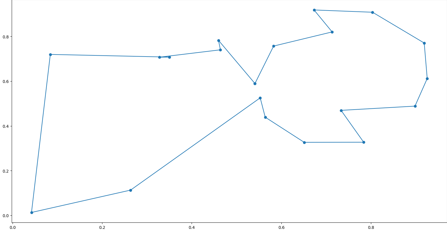Cool! We managed to get a Hamiltonian cycle with a weight of 3.8353886994528303. Running for more iterations makes the algorithm converge to cheaper solutions. Now, for our final problem, we’ll look at the Knapsack problem\

Knapsack

The Knapsack problem (0-1 Knapsack, to be more precise) is also a relatively simple problem that doesn’t have a known exact polytime solution. Suppose you have a list of items, where each item has a value, which is a positive number, and a weight, which is also a positive number. For each item, you can either take it or not take it. Because you can only carry a limited weight, the sum of the weights of your items cannot exceed a certain threshold, such as 20kg. You goal is to take the items that yield the maximum value, without exceeding the threshold. For example, if you have the following items: Gold bar - 100$ - 5kg Necklace - 60$ - 3kg Ring - 10$ - 0.5g Bracelet - 70$ - 2kg With a limitation of 6kg, you can, for example, take the gold bar and the ring, yielding a value of 110$ with a weight of 5+0.5 = 5.5kg. You can also take the necklace, ring, and bracelet yielding a value of 140$ with the same weight of 5.5kg. Let’s solve the problem! We start by defining our chromosomes as Boolean vectors, where a true at index i tells us to take item i, and a false tells us to not take it:

struct Knapsack {
// True if we include the item in the knapsack and
// false otherwise
items: [bool; NUM_ITEMS],
}

Now, let’s implement the Chromosome trait. To generate a random Knapsack, we just make a random vectors of 0s and 1s:

// Generate a random (possibly weight-exceeding) knapsack
fn random() -> Self {
	let mut rng = thread_rng();
	let dist = Bernoulli::new(0.5).unwrap();
	// Generate a vector of NUM_ITEMS random booleans
	let items: Vec<bool> = dist.sample_iter(&mut rng).take(NUM_ITEMS).collect();
	
	Knapsack {
		items: items.try_into().unwrap(),
	}
}

This might seem like a slightly weird choice, since after all nothing stops the random vector from exceeding the weight limitation. This is true, but eventually, because exceeding the weight limitation makes the fitness function low (as we’ll see later), the population will evolve in the direction of valid knapsacks. Now, the mutation operation is simply a bit flip (or multiple bit flips, depending on how many mutations occurred):

fn mutate(&self, mutations: &[bool]) -> Self {
	let mut new_knapsack = Knapsack { items: self.items };
	
	for i in 0..NUM_ITEMS {
		// If this bit has mutated, flip it
		if mutations[i] {
		new_knapsack.items[i] = !new_knapsack.items[i];
		}
	}
	
	new_knapsack
}

Again, this might result in invalid knapsacks, but the natural selection process cancels that out. Now, the fitness function is defined as the sum of values if the knapsack doesn’t exceed the weight limitation, and as -1 otherwise:

fn fitness(&self) -> f64 {
	// Sum all of the weight values
	// Stop summing and return a negative value if we exceed the maximum weight allowed
	let mut value_sum = 0f64;
	let mut weight_sum = 0f64;
	// Knapsack data (weights and values)
	let data = KnapsackData::new();
	let (values, weights) = (data.values, data.weights);
	
	for i in 0..NUM_ITEMS {
		// If the knapsack contains the item
		if self.items[i] {
			value_sum += values[i];
			weight_sum += weights[i];
		}
	
	// We exceeded the maximum allowed weight
		if weight_sum > MAX_WEIGHT {
			return -1f64;
		}
	}
	
	value_sum
}

The KnapsackData structure contains the weights and the values of all items. Finally, for the crossover operation, we swap a subsequence of the bits between the two parents:

fn crossover(x: Self, y: Self) -> (Self, Self) {
	let mut new_x = Knapsack { items: x.items };
	let mut new_y = Knapsack { items: y.items };
	
	// Exchange 2/3 of the bits
	for i in 0..2 * (NUM_ITEMS / 3) {
		let tmp = new_x.items[i];
		new_x.items[i] = new_y.items[i];
		new_y.items[i] = tmp;
	}
	
	(new_x, new_y)
}

Awesome! Let’s run it:

let mut run = Run::<Knapsack>::new(200, 0.05, 0, N_POP, NUM_ITEMS, evolve::Selection::Softmax);

let history = run.begin();

for (knapsack, value) in history {
	println!("{}\t{}", knapsack, value);
}

Note that here, instead of generating the selection distribution using a probability proportional to the place of the chromosome, we use the softmax function. On the following items:

Values: 3, 2, 4, 3.5, 7.2, 5.9, 0.7, 8, 6, 10, 1, 3.1
Weights: 8, 2, 1, 3.5, 5.7, 3, 8, 9, 2.3, 5.5, 6, 0.2

We get the following knapsack after 200 iterations:

1 2 4 5 8 9 11 38.2

The numbers shown are the indexes of the items we want to include in the knapsack. The final number 38.2 is the total value.

Conclusion

Writing this post was very interesting, and I learned a lot from it. I always thought that approximation algorithms for problems such as the TSP were very theoretical and complicated. Making such as algorithm and seeing it in action is very cool! Additionally, I think that taking inspiration from biological concepts is a really cool and interesting idea. You can find the library shown in this post, along with all the examples here. Thanks for reading :) Yoray

References

Jenna Carr, “An Introduction to Genetic Algorithms”