Ant Colony Optimization in Golang!
Introduction
Several months ago, I wrote about implementing Genetic Algorithms in Rust to solve optimization problems. In today’s post, we are going to use another such nature-inspired algorithm called Ant Colony Optimization (ACO) to solve a classic NP-Complete problem (which we also tackled last post): The Traveling Salesman Problem (TSP). Unlike last post, we’re going to implement the algorithm in Go (instead of Rust), mostly because I want to learn more about the language :) Note: If you are unfamiliar with the TSP, you can find an explanation on it in the previous post or in the Wikpedia page on the TSP. Note 2: The code for this post is available here
Ant Colony Optimization
History
In the early 90s, to research the communication among ants, Biologists ran an interesting experiment called the Double Bridge Experiment. In the experiment, an anthill and a food source are connected with two different bridges, as shown below.
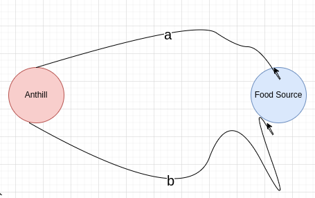
The length of the first bridge is labeled a and the length of the second bridge is labeled b (you’re not wrong if this setup reminds you of a graph). The anthill, being an anthill, houses many ants; the goal of the experiment is to test how the (ratio between the) lengths of the bridges affects the number of ants walking on each bridge. When the bridges were of equal length (i.e. a=b), the percentage of ants walking on each bridge was roughly the same (there were, of course, some fluctuations, due to ants having some randomness to their behaviour). When one bridge was longer than the other (e.g. a=2b), however, the results changed drastically! The amount of ants that chose to walk on the short bridge was greater. What’s more, as time progressed, the phenomenon had “converged”, until almost all ants chose to walk on the short bridge. To understand this strange behaviour, we should look into the communication mechanism of ants. Unlike humans or other animals, whose communication with each other is audiatory (i.e. based on sound) and visual, ants communicate using the sense of smell. When ants walk, they spread a chemical called pheromone on the ground. Other ants can then know where their peers walked, and walk in the same path (this is how so-called ant highways are formed). In the double bridge experiment, initially both bridges do not have any pheromone on them, so the ants choose a bridge randomly. The ants that choose the short bridge would get to the food source faster than their peers who chose the long bridge. The means that they would also start making the trip back to the anthill first. In other words, the round-trip time of the ants that chose the shorter bridge is shorter than the round-trip time of the ants that chose the longer bridge. This implies that the ants who chose the shorter bridge would deposit their pheromone on the shorter bridge before the ants who chose the long bridge do so on the long bridge. The ants now at the anthill, faced with the choice of which bridge to walk through, would have a greater probability of choosing the short bridge, since it has a larger amount of pheromones on it. Eventually, more and more pheromones accumulate on the short bridge, and almost all ants would choose it rather than the long bridge. In the next section, we’ll translate the result of this experiment into a heuristic that can be used to solve computational problems.
Developing a Heuristic
We begin by noting the explore/exploit behaviour of the ants in the experiment: at first, when there wasn’t yet a large amount of pheromone deposited on either bridge, the ants chose a bridge randomly, exploring their environment. As time progressed, however, more ants choose the short bridge (since there was a larger amount of pheromone on it), exploiting the knowledge the colony had gathered. As in the experiment, we will set our (artificial) ants in a graph, with each ant being on a node in the graph at each timestep. Each edge of the graph contains an amount of pheromone; we denote with tau_{ij} the amount of pheromone on the edge (i, j). Suppose that an ant A is now at node v. How does it decide which node to go to next? A trivial answer would be to compute a probability distribution over the nodes in v’s neighbourhood using only the pheromones (we must also normalize by dividing by the sum of all pheromones):
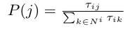
Where N^{i} is the neighbourhood of node i. In other words: the higher the pheromone on an edge is, the more likely we are to go to the node connecting that edge with i. The problem with this approach is that the ants are very likely to get into a feedback loop and reach a suboptimal solution, since they don’t have a notion of some edges being, heuristically, better than others. To add this capability, we also introduce a heuristic value eta_{ij} to each edge (i, j) that is decided upon before running the algorithm. In TSP, for example, we’ll set it to be inversely proportional to the length of the edge (so that edges with lower costs have greater heuristics). Our final probability distribution is therefore as below.
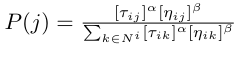
Alpha and beta are hyperparameters that control how much weight we give to the pheromones vs. the heuristics. Typically, beta is set to be greater than alpha (so that the heuristics have more weight than the pheromones), to prevent the algorithm from getting stuck in a feedback loop, leading to a suboptimal solution. Another point I did not mention in the previous section is the evaporation of pheromones. The pheromones, being a liquid, slowly evaporate from the bridges, decreasing the amount of pheromone on each bridge. This also helps prevent the algorithm from reaching a suboptimal solution. To implement this, we will decay each pheromone exponentially; for each timestep t:
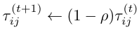
Where rho is a hyperparameter controlling the rate of decay
The Algorithm
Though there are multiple algorithms based on the Ant Colony heuristic, the one we’ll use in this post is called Ant System. The algorithm shown below was originally presented by Dorigo et al. in the paper “The Ant System: Optimization by a colony of cooperating agents” for the purposes of solving the TSP, though it can be adapted to handle other optimization problems.
- Place each ant on a random node in the graph
- Repeat the following until you get to a desired amount of accuracy:
- Let each ant complete a hamiltonian cycle (pass through all other nodes and return to the one it was initially on), where ants choose an edge according to the probability distribution from the previous section
- Evaporate the current pheromones
- Let each ant deposit its pheromones on the edges it passed, where an ant depsoits pheromones inversely proportional to the length of the hamiltonian cycle it completed. This ensures that shorter cycle (which are better) are given more weight
The Implementation
Ant Colony
We’re going to start off by creating a struct called AntColony:
1
2
3
4
5
6
7
8
9
10
11
12
13
14
type AntColony struct {
	// The construction graph G = (C, L) of the problem
	// C is the set of components (e.g. cities in TSP)
	// and L is the set of connections (in TSP, for example, all pairs of cities are connected)
	constructionGraph Graph
	// Pheromones on connections - this indicates to the ants how good the connection is
	Pheromones [][]float64
	// We can also have heuristic information on the arcs - for TSP, this is the repriocorial of the cost of the edge
	heuristics [][]float64
	// The ants
	ants []Ant
	// Number of ants
	num_ants uint
}
As you might’ve guessed from the previous sections, to run ACO algorithms we first have to translate our problem into a graph. For TSP, this is trivial: the graph is just the instance of the problem. We keep this graph in the constructionGraph field. The Graph type is a very simple implementation of a graph, shown below.
1
2
3
4
5
6
7
8
9
10
11
12
13
// An edge (a, b) in an undirected graph G
type Edge struct {
	A uint
	B uint
}

// A graph G = (V, E)
type Graph struct {
	// The list of node indices V
	Nodes []uint
	// We store the edges in a slice: entry i in the slice is the list of all edges from vertex i
	Edges [][]Edge
}
The edges are stored in slice of slices, where the i-th entry of the Edges slice is the all the edges connected to node i. The nodes are treated as unsigned integers. Going back to the AntColony struct, we track a list of our ants in a slice called ants. Each ant is of type, well, Ant:
1
2
3
4
5
6
7
8
9
10
// An individual ant
type Ant struct {
	// The index of the current component, i.e. the current vertex in the construction graph
	currComponent uint
	// Which components has this ant already visited?
	// Used to define constraints
	memory map[uint]bool
	// We also store the explicit edges to compute the pheromones
	tour []Edge
}
The ant keeps track of which node it currently is on the graph, which nodes it has visited (so that it knows not to visit the same nodes multiple times), and which edges it used in the hamiltonian cycle. For the ant colony to solve a problem, it needs a way to (a) construct a graph based on the instance of the problem and (b) initialize the pheromones and heuristics on all edges (see the previous section). To implement this, we create an interface ACOptimizable (shown below) that problems must implement.
1
2
3
4
5
6
7
8
9
10
11
type ACOptimizable interface {
	// How to construct a graph from this problem?
	ConstructGraph() Graph
	// How should the pheromones be initialized? For example,
	// for TSP, a common heuristic is to initialize all pheromones as m / C^{nn}, where m
	// is the number of ants, and C^{nn} is
	// the length of a cycle constructed with a nearest neighbour (greedy) heuristic
	InitPheromones(num_ants uint) [][]float64
	// Similarily, how should the heuristics be initialized?
	InitHeuristics() [][]float64
}
Let’s start doing something with those definitions!
Initializing an Ant Colony
The first function will initialize an AntColony from an ACOptimizable problem:
1
2
3
4
5
6
7
8
9
10
11
12
13
14
15
16
17
18
19
20
21
// Construct a new ant colony for an ACOptimizable problem with num_ants ants
func NewAntColony(problem ACOptimizable, num_ants uint) *AntColony {
	colony := new(AntColony)
	colony.constructionGraph = problem.ConstructGraph()
	colony.Pheromones = problem.InitPheromones(num_ants)
	colony.heuristics = problem.InitHeuristics()
	colony.num_ants = num_ants
	colony.ants = make([]Ant, 0)

	// Initialize all the ants
	for i := 0; i < int(num_ants); i++ {
		// Generate a random city=component
		rand_component := rand.Intn(len(colony.constructionGraph.Nodes))
		// Append the ant to the ant list
		ant_memory := make(map[uint]bool)
		//ant_memory[uint(rand_component)] = true
		colony.ants = append(colony.ants, Ant{uint(rand_component), ant_memory, make([]Edge, 0)})
	}

	return colony
}
The number of ants is specified by the user; the more ants there are, the faster the solution will be found (in most cases). Each ant is placed in a random node. The ant’s memory & tour are both initialized as empty maps and slices, respectively.
Implementing the AntSystem Algorithm
Now that we can initialize an ant colony, let’s use it to solve some problems! This is done using the function RunSimulation:
1
2
3
4
5
6
7
8
9
10
11
12
13
14
15
16
17
func (colony *AntColony) RunSimulation(num_iters int) {
	for i := 0; i < num_iters; i++ {
		// Have each ant complete a cycle
		for i := 0; i < int(colony.num_ants); i++ {
			colony.ants[i].DoCycle(colony)
		}

		// Evaporate the pheromones to avoid converging on a suboptimal solution
		colony.EvaporatePheromones()
		// Update the pheromones from all the ants
		for _, ant := range colony.ants {
			ant.DepositPheromones(colony)
			// We want a clean slate for our ant in the next iteration
			ant.ResetSolution(colony)
		}
	}
}
The user chooses a number of full iterations to run the algorithm for (you can think of this like the number of generations in Genetic Algorithms or the number of epochs when training Neural Nets). In each iteration, all the ants complete a cycle on the graph using the function DoCycle, which we will get to shortly. Afterwards, the pheromones currently on the graph are evaporated, and all the ants deposit their pheromone (the ResetSolution function resets the state of the ant before running the next iteration).
Completing a Cycle
The DoCycle function is shown below:
1
2
3
4
5
6
7
8
9
10
11
12
13
14
15
16
17
18
19
20
21
22
23
24
25
26
27
28
29
30
31
32
33
34
35
36
37
38
39
40
41
42
43
44
45
46
47
48
func (ant *Ant) DoCycle(colony *AntColony) {
	ant.memory = make(map[uint]bool)
	ant.tour = make([]Edge, 0)
	initLocation := ant.currComponent

	// Our tour should be as long as the number of vertices
	for len(ant.tour) != len(colony.constructionGraph.Nodes) {
		ant.memory[ant.currComponent] = true

		// What is the probability of going to each edge in our neighbourhood?
		// For simplicity, we also track the probabilities of nodes not in our neighbourhood (and set them to 0)
		weights := make(map[uint]float64)
		// We track the sum of the edge scores so that we can normalize by it
		// and convert it to a valid probability distribution
		denom := 0.0

		for _, edge := range colony.constructionGraph.Edges[ant.currComponent] {
			if !ant.memory[edge.B] && edge.A != edge.B {
				// The score for this edge is affected by the current amount of pheromones on it
				// and its heuristic (e.g. in TSP the heuristic is inversely proportional to the weight of the edge)
				score := math.Pow(colony.Pheromones[edge.A][edge.B], alpha) * math.Pow(colony.heuristics[edge.A][edge.B], beta)
				weights[edge.B] = score
				denom += score
			} else {
				// If this edge either (1) goes from the current node to itself or (2) the node it goes to has
				// already been visited, set its probability to 0
				weights[edge.B] = 0
			}
		}

		// Normalize the scores to convert into a valid probability distribution
		for dest := range weights {
			weights[dest] /= denom
		}

		// Sample one of the edges according to the probability distribution
		dest := weightedSampling(weights)
		edge := Edge{A: ant.currComponent, B: uint(dest)}
		// Go through the edge and change our current location
		ant.currComponent = edge.B
		ant.tour = append(ant.tour, edge)
		// If we only have one edge left, we mark the initial location (the start of the cycle)
		// as unvisited again
		if len(ant.tour) == len(colony.constructionGraph.Nodes)-1 {
			ant.memory[initLocation] = false
		}
	}
}
The function stores the initial node the ant was in to a variable initLocation, and then runs in a while loop until the length of the ant’s tour (the number of edges) is the same as the number of nodes in the graph (a Hamiltonian Cycle must have this property; with less edges and it would not reach all nodes, and with more edges it would have to visit certain nodes multiple times). Inside the while loop, we compute a weight for each of the nodes in our current node’s neighbourhood:
1
2
3
4
5
6
7
8
9
10
11
12
13
14
15
16
17
18
19
20
21
22
23
24
25
26
ant.memory[ant.currComponent] = true
// What is the probability of going to each edge in our neighbourhood?
// For simplicity, we also track the probabilities of nodes not in our neighbourhood (and set them to 0)
weights := make(map[uint]float64)
// We track the sum of the edge scores so that we can normalize by it
// and convert it to a valid probability distribution
denom := 0.0

for _, edge := range colony.constructionGraph.Edges[ant.currComponent] {
	if !ant.memory[edge.B] && edge.A != edge.B {
		// The score for this edge is affected by the current amount of pheromones on it
		// and its heuristic (e.g. in TSP the heuristic is inversely proportional to the weight of the edge)
		score := math.Pow(colony.Pheromones[edge.A][edge.B], alpha) * math.Pow(colony.heuristics[edge.A][edge.B], beta)
		weights[edge.B] = score
		denom += score
	} else {
		// If this edge either (1) goes from the current node to itself or (2) the node it goes to has
		// already been visited, set its probability to 0
		weights[edge.B] = 0
	}
}

// Normalize the scores to convert into a valid probability distribution
for dest := range weights {
	weights[dest] /= denom
}
We start by marking the current node as visited, and then we weight the edges according to the formula we derived in the “Developing a Heuristic” section:
Alpha and Beta are defined as follows:
1
2
3
4
// Pheromone weight
const alpha = 1.0
// Heuristic weight
const beta = 3.0
Note that for nodes that are either (1) not in our neighbourhood or (2) have already been visited we set the probability to 0. We finally normalize the scores by dividing by their sum to convert them into a valid probability distribution. With this probability distribution, we sample a node to go to, travel through the corresponding edge, and append it to our tour:
1
2
3
4
5
6
// Sample one of the edges according to the probability distribution
dest := weightedSampling(weights)
edge := Edge{A: ant.currComponent, B: uint(dest)}
// Go through the edge and change our current location
ant.currComponent = edge.B
ant.tour = append(ant.tour, edge)
The weighted sampling function isn’t included here since it’s not very interesting - it just samples a node from a map[uint]float64 (the uints are the nodes), treating the float64s as probabilities. Note that if we only have one edge left (i.e. we’ve already visited all nodes), we need to mark the initial location of the ant (the start of the cycle) as unvisited, since otherwise the loop would assign probability 0 to all nodes as they have all been visited, and the cycle would never end:
1
2
3
4
5
// If we only have one edge left, we mark the initial location (the start of the cycle)
// as unvisited again
if len(ant.tour) == len(colony.constructionGraph.Nodes)-1 {
	ant.memory[initLocation] = false
}
This ensures that, in the next iteration, the ants would choose the start of the cycle as the end (since it’s the only unvisited node).
Pheromone Evaporation
Evaporating the pheromones is quite simple; as discussed in the “Developing a Heuristic” section, it’s implemented with exponential decay:
1
2
3
4
5
6
7
func (colony *AntColony) EvaporatePheromones() {
	for i := 0; i < len(colony.constructionGraph.Nodes); i++ {
		for j := 0; j < len(colony.constructionGraph.Nodes); j++ {
			colony.Pheromones[i][j] *= (rho)
		}
	}
}
Where rho controls the rate of decay:
1
2
// Exp. decay rate for the pheromone
const rho = 0.5
Pheromone Deposition
When depositing the pheromones, we’d like ants that had completed shorter tours to deposit more pheromones, so that they would cause more ants in the next iteration to follow in their tracks. As mentioned earlier, this is done by having the amount of pheromone deposited by each ant be inversely proportional to the length of the tour completed by the ant:
1
2
3
4
5
6
7
8
9
10
11
func (ant *Ant) DepositPheromones(colony *AntColony) {
	tourCost := 0.0

	for _, edge := range ant.tour {
		tourCost += 1.0 / colony.heuristics[edge.A][edge.B]
	}

	for _, edge := range ant.tour {
		colony.Pheromones[edge.A][edge.B] += 1.0 / tourCost
	}
}
The TSP
Implementing the Interface
Great! Now that we’ve implemented the basic Ant System algorithm, let’s try it on the TSP. To do that, we’ll implement the ACOptimizable interface on the TSP. Recall that it is defined as follows:
1
2
3
4
5
6
7
8
9
10
11
type ACOptimizable interface {
	// How to construct a graph from this problem?
	ConstructGraph() Graph
	// How should the pheromones be initialized? For example,
	// for TSP, a common heuristic is to initialize all pheromones as m / C^{nn}, where m
	// is the number of ants, and C^{nn} is
	// the length of a cycle constructed with a nearest neighbour (greedy) heuristic
	InitPheromones(num_ants uint) [][]float64
	// Similarily, how should the heuristics be initialized?
	InitHeuristics() [][]float64
}
We define the TSP with the below structure, which stores the graph, and the weights on the edges as a slice of slices:
1
2
3
4
type TravelingSalesman struct {
	graph   antcolony.Graph
	weights [][]float64
}
As mentioned before, constructing a graph from the problem is trivial, since the problem is already defined on a graph (although in other graph problems some transformations might still be needed):
1
2
3
func (tsp *TravelingSalesman) ConstructGraph() antcolony.Graph {
	return tsp.graph
}
We initiate the pheromones to be inversely proportional to the greedy solution (i.e. start on a random node and each time pick the nearest node, until a cycle is completed):
1
2
3
4
5
6
7
8
9
10
11
12
13
14
15
func (tsp *TravelingSalesman) InitPheromones(num_ants uint) [][]float64 {
	pheromones := make([][]float64, 0)

	for i := 0; i < len(tsp.graph.Nodes); i++ {
		pheromone := make([]float64, 0)

		for j := 0; j < len(tsp.graph.Nodes); j++ {
			pheromone = append(pheromone, float64(num_ants)/tsp.greedySolution())
		}

		pheromones = append(pheromones, pheromone)
	}

	return pheromones
}
The greedySolution function is shown below.
1
2
3
4
5
6
7
8
9
10
11
12
13
14
15
16
17
18
19
20
21
22
23
24
25
26
27
28
29
30
31
32
33
34
35
36
37
38
39
// Used when computing the pheromones for ACO: the peromones are set to the repricorial of the length of a
// hamilitonian cycle found with a greedy nearest-neighbour search
func (tsp TravelingSalesman) greedySolution() float64 {
	tour := make([]antcolony.Edge, 0)
	initComponent := uint(rand.Intn(len(tsp.graph.Nodes)))
	currComponent := initComponent
	memory := make(map[uint]bool)
	tourCost := 0.0

	// Our tour should be as long as the number of vertices
	for len(tour) != len(tsp.graph.Nodes) {
		var bestEdge antcolony.Edge
		bestWeight := math.Inf(1)

		for _, edge := range tsp.graph.Edges[currComponent] {
			memory[currComponent] = true

			if !memory[edge.B] && edge.A != edge.B {
				if tsp.weights[edge.A][edge.B] < bestWeight {
					bestEdge = edge
					bestWeight = tsp.weights[edge.A][edge.B]
				}
				bestEdge = edge
			}
		}

		// Go through the edge and change our current location
		currComponent = bestEdge.B
		tourCost += tsp.weights[bestEdge.A][bestEdge.B]
		tour = append(tour, bestEdge)
		// If we only have one edge left, we mark the initial location (the start of the cycle)
		// as unvisited again
		if len(tour) == len(tsp.graph.Nodes)-1 {
			memory[uint(initComponent)] = false
		}
	}

	return tourCost
}
You might wonder why the pheromones are initialized this way. If the pheromones were too low, the algorithm would be much more sensitive to the heuristics, making the algorithm more similar to a greedy search, and harming the explorative phase. If the pheromones were too high, the algorithm would try too many possible options, harming the exploitative phase; Therefore, initializing the pheromones to be inversely proportional to a known solution is a nice middle ground. As discussed previously, the heuristic on each edge is set to be inversely proportional to the cost of the edge, making the algorithm favour shorter edges:
1
2
3
4
5
6
7
8
9
10
11
12
13
14
15
func (tsp *TravelingSalesman) InitHeuristics() [][]float64 {
	heuristics := make([][]float64, 0)

	for i := 0; i < len(tsp.graph.Nodes); i++ {
		heuristic := make([]float64, 0)

		for j := 0; j < len(tsp.graph.Nodes); j++ {
			heuristic = append(heuristic, 1.0/(tsp.weights[i][j]+1e-8))
		}

		heuristics = append(heuristics, heuristic)
	}

	return heuristics
}
We add a small number when dividing by the cost of the edge to not divide by zero.
Running the Algorithm
Awesome! We’ve written everything we need to run the algorithm, so all we need to do is generate an instance of the problem. To do this, I’ve used the following Python code:
1
2
3
4
5
6
7
8
9
10
11
12
13
14
15
16
17
18
19
20
21
22
23
24
25
import random
import numpy as np
import matplotlib.pyplot as plt

random.seed(1337)

# Generate 20 random points
points = [[random.random(), random.random()] for _ in range(20)]
# Find the distance matrix
dist_mat = []

for i in range(20):
    dists = []

    for j in range(20):
        dists.append(np.linalg.norm(np.array(points[i]) - np.array(points[j])))

    dist_mat.append(dists)

with open("dist_mat", "w") as f:
    for row in dist_mat:
        for dist in row:
            f.write(f"{dist} ")

        f.write("\n")
The script generates 20 random points, and outputs the distances between them to a file dist_mat. To run the ACO algorithm on this file, we use the following code:
1
2
3
4
5
6
7
8
9
10
11
12
13
14
15
func main() {
	graph := newCompleteGraph(20)
	weights := weightsFromFile("./dist_mat")

	tsp := TravelingSalesman{graph: graph, weights: weights}

	antColony := antcolony.NewAntColony(&tsp, 200)
	antColony.RunSimulation(100)

	cycle := antColony.GetSolution()

	for _, edge := range cycle {
		fmt.Printf("(%d, %d)\n", edge.A, edge.B)
	}
}
The newCompleteGraph function generates a fully-connected graph with 20 nodes, and the weightsFromFile function loads the weights from the file output by the Python script. Both function are not very interesting, so I do not include their implementation here. We then initialize a new TSP from the graph and the weights, and run the ACO algorithm with 200 ants for 100 iterations. Finally, we print the solution. The GetSolution function runs a new ant on the graph, and returns the ant’s tour:
1
2
3
4
5
func (colony *AntColony) GetSolution() []Edge {
	colony.ants[0].DoCycle(colony)

	return colony.ants[0].tour
}
This is based on the fact that after the ant colony had been trained, the state of the pheromones will likely make new ants’ tours be good solutions to the TSP. Running the program (which took 0.3 seconds), we get the following output (the output will change each run due to the randomness of the algorithm):
1
2
3
4
5
6
7
8
9
10
11
12
13
14
15
16
17
18
19
20
(11, 12)
(12, 0)
(0, 18)
(18, 1)
(1, 3)
(3, 10)
(10, 13)
(13, 6)
(6, 15)
(15, 2)
(2, 7)
(7, 9)
(9, 14)
(14, 4)
(4, 5)
(5, 19)
(19, 8)
(8, 17)
(17, 16)
(16, 11)
Plotting it on the points:
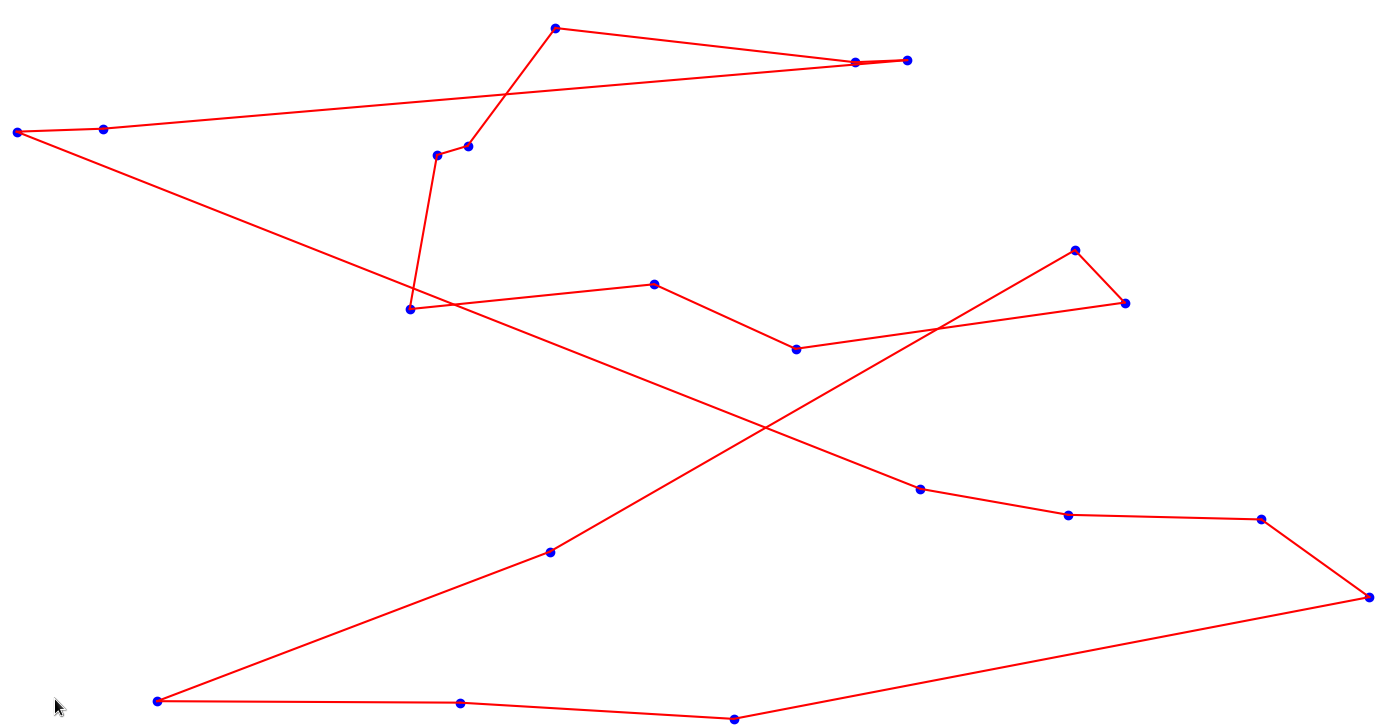
Great! It seems like a pretty good solution.
Conclusion
In this post, we’ve implemented the Ant System algorithm in Go. As I mentioned in the previous post, I find the idea of using ideas from Biology to solve computational problems very compelling. Go lended itself well for the implementation and I’ve learned some more about the language by doing this. Note that Ant System is not the only algorithm based on the ACO meta-heuristic: some other notable algorithms are Ant Colony System (ACS), Elitist Ant System, and more. ACO is also not limited to graph problems, although, to apply ACO to such problems, we must first construct a graph representing the problem (e.g. in the knapsack problem the nodes would represent items).
Thanks for reading :)