Implementing Merkle Trees in Go

Introduction

Say you and I have access to some source of truth where data is posted every once in a while – the classic example would be something like Bitcoin, where a new block containing 1000s of transactions is published to the chain every ~10 minutes. It would be useful if we could make backed-up statements about this public data: for example, I could prove to you that I paid 10 BTC to Alice in block X, and you could verify this proof and grant me some service in exchange. Each Bitcoin block stores all of its transactions, so the trivial solution would be to have my proof simply consist of the transaction itself and the block height: I paid Alice 10 BTC in block X. Verifying this proof entails looking up block X, and checking whether the transaction I paid Alice 10 BTC indeed appears in the transactions contained there. This, however, introduces 2 problems:

1. To verify this proof, you would have to iterate over each item in the dataset (in the Bitcoin usecase, this is not much of a problem, as a block contains at most 1000s of transactions, but in other cases, where the dataset is billions of items large, this would be more problematic).
2. Each block would have to store a lot of extra bytes, which would drastically increase bandwidth and storage costs for non-full nodes that want to perform such verification, i.e. nodes that don’t store the entire blockchain locally.

But there’s another way. In 1988, Ralph Merkle invented a data structure that:

• Supports proofs with logarithmic size and verification time: producing and verifying a proof that an item is included in a dataset of N items requires O(log N) time, and:
• The size of data that needs to be stored publicly for verification is constant: something like 32 bytes, even for a dataset containing a trillion items.

Note that for generating proofs, you still need to have access to all of the items. However, this lines up with the notion, which is true in most cases, that provers should have to work harder than verifiers in order to prove a statement. This might seem impossible at first, but the underlying math is actually quite simple and elegant, and the base variant can be implemented in about a 100 lines of Go!

Merkle Trees 101

Judging by the “constant 32 bytes” thing, you’d be right if you guessed that hash functions are involved somehow, though it’s not immediately obvious how they should be used. A good first step is to simplify the problem – what if our dataset contained only 2 items: a and b?

The Simplified Case

In this case, we could first hash these items using some hash function H to get H(a) = A and H(b) = B. Then, we could concatenate A and B, and hash them: AB = H(A || B), where || denotes concatenation. This is called a commitment to our data, in the following sense:

Some party can claim that the dataset contains items a and b, and not any other items, and post this commitment. Assuming a collision-free hash function, no other items will produce the same commitment. Anyone who has access to the data can verify this commitment by going through the same steps the committer just did, and checking whether the final hash they get is equal to the one posted by the committer.

This is all well and good, but how does it help us solve the original problem? Graphically, we can see that the commitment process induces a tree structure:

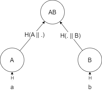
The crucial property here that lets us do proofs of inclusion over this tree, is the fact that if you have both A and B, you can compute AB. Therefore, to prove that item a, for example, is included in the tree, a Prover can send the verifier the following 3 items:

1. The root of the tree, AB
2. The item a whose existence the Prover wants to prove
3. The hash B

These 3 items give the Verifier everything they need to verify the existence of a, which they can do as follows:

• Hash a to get A = H(a)
• Hash the A computed by the Verifier and the B sent by the Prover to get AB' = H(A || B)
• Accept the proof if and only if AB' = AB, where AB is the root sent by the Prover

That’s it! The 3 items sent by the Prover are called a Merkle Proof. Note that the proof is only as secure is the root sent: an adversarial prover can always construct a Merkle tree over another dataset containing a, and send the proof over this tree, and the verifier would have no way of knowing the proof is for a dataset other than the original one. For this reason, Merkle Trees are typically used in cases where the Merkle Root is agreed upon publicly: for example, when the root is posted by a trusted third party, such as a newspaper, or is agreed upon in a decentralized system using consensus, as in the case of Bitcoin, so that the prover cannot post a false Merkle Tree.

The General Case

Generalizing the algorithm we constructed in the previous case to an arbitrary number of items is much simpler than it sounds, and is based mostly on a divide-and-conquer approach. If you have a dataset of, say, 4 items, a, b, c, and d, you first split them into 2 groups: a and b, and c and d. Then, you run the 2-item algorithm over each 2-item group:

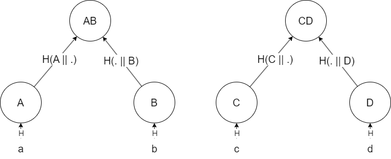
And compute the root of the tree as ABCD = H(AB || CD):

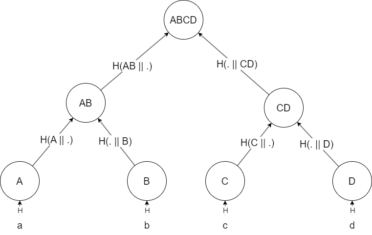
Note that the new root, ABCD, represents a commitment over a, b, c, and d. If one of these items would change, the commitment would no longer be valid. Proving that an item exists in this larger tree is similar to the 2-item case, but the proof requires sharing an additional hash. To prove that a exists in this tree, for example, the prover would send the following data:

1. The root ABCD (as in the simplified case).
2. The item a (as in the simplified case).
3. The hash B, as in the simplified case.
4. With the data sent so far, the verifier can reconstruct AB, but not the root ABCD. Therefore, the prover also sends CD. The verifier verifies this proof as follows:
   • Compute A = H(a).
   • Compute AB = H(A || B).
   • Compute ABCD' = H(AB || CD).
   • Accept the proof if and only if ABCD' = ABCD. Extending this idea to even more items is similar. Note how the proof size scales logarithmically WRT the number of items in the dataset, and the data that needs to be posted publicly, the root, is only as large as the digest size, so 32 bytes for SHA256 for example. If you’d have a billion items, the proof would only consist of log_2 (10^9) == 10 hashes, and the root would still only be 32 bytes!

Implementation

Constructing a Tree

Now that we understand how basic Merkle Trees work, we can write our first implementation in Golang (you can find the complete code used in this post here). We represent a Merkle Tree using its root:

type MerkleTree struct {
	root merkle_node
}

Each node contains a digest (which is computed as H(left child's digest || right child's digest)), and a pointer to each of its children:

const DIGEST_SIZE = 32

type merkle_node struct {
	// We hold the hash of some data
	data [DIGEST_SIZE]byte
	// Point to our left and right children
	left  *merkle_node
	right *merkle_node
}

To construct the tree from some set of data, we use recursion. We have two base cases: one for the case we get an empty set of data as input (this only happens when the dataset size is not a power of two), and another for the case we get a single item of data as input, in which case we simply hash the item and return it:

// Construct a Merkle Tree using some data
func NewMt(data [][]byte) *MerkleTree {
	// If there's no data here, return nil
	if len(data) == 0 {
		return nil
	}
	// Recursion... if we only have one piece of data, hash it, and return the resulting leaf
	if len(data) == 1 {
		leaf := merkle_node{
			sha256.Sum256(data[0]),
			nil,
			nil,
		}
		tree := MerkleTree{leaf}

		return &tree
	}
	...
}

Otherwise, we split the dataset in half, call the NewMt function on each half, compute the digest of the current node by concatenating its children’s digests, and returning the result:

// Construct a Merkle Tree using some data
func NewMt(data [][]byte) *MerkleTree {
	...
	// Otherwise, you construct the Merkle Trees corresponding to the two halves of the data
	left := NewMt(data[:len(data)/2])
	right := NewMt(data[len(data)/2:])
	// and set the data of this node to be H(left.root || right.root)
	combined := append(left.root.data[:], right.root.data[:]...)
	root_data := sha256.Sum256(combined)
	// construct the root from what we just computed
	root := merkle_node{
		root_data,
		&left.root,
		&right.root,
	}
	tree := MerkleTree{root}

	return &tree
}

You might wonder whether splitting the dataset in half, so that the resulting tree is balanced, is always the right approach. Indeed, the assumption here is that provers want to generate proofs of inclusion over all items uniformly, i.e. the aren’t items for which proofs are generated more frequently. If, say, 90% of the proofs were generated for item a, we could construct the tree as follows:

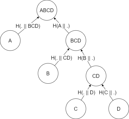
Then, proofs for A would require sending only one additional hash, instead of two: BCD. For small datasets the difference is negligible, but when you have millions of items and send thousands of proofs over the wire per second, this starts to matter. I didn’t implement this type of unbalanced tree in the code, but it’s worth keeping in mind :)

Inclusion Proofs

Recall that the proof is comprised of the sibling of every node in the path from the root to the leaf. In our implementation, we will also store the side (left or right) of every such sibling, since otherwise the verifier can’t reconstruct the root:

type MerkleProof struct {
	// The list of hashes that constitutes the proof
	hashes [][DIGEST_SIZE]byte
	// The side each hash is on (is it the right child or the left child)
	left []bool
}

Generating a proof starts with finding a path from the root of the tree to the leaf whose inclusion we want to prove:

// Generate a proof that some item is a part of the Merkle tree
func (tree *MerkleTree) Prove(item []byte) *MerkleProof {
	// First, we want to find to find the leaf corresponding to the item inside the tree
	path := tree.root.search(item)
	...
}

// Find a path from the root of the provided Merkle tree to the leaf containing the hash of the item
func (root *merkle_node) search(item []byte) []*merkle_node {
	// Base case -- the provided tree is a leaf
	if root.left == nil && root.right == nil {
		// If the leaf contains the hash of the item: great
		if root.data == sha256.Sum256(item) {
			return []*merkle_node{root}
		} else {
			return nil
		}
	}
	// Search in the left and right subtrees
	left := root.left.search(item)
	right := root.right.search(item)
	// If the left is not nil, we append the current root to the path it found
	if left != nil {
		path := append(left, root)

		return path
	} else if right != nil {
		// Same thing for right
		path := append(right, root)

		return path
	}
	// If it doesn't exist in either subtree, it isn't in the tree at all
	return nil
}

Afterwards, for each node in the path, we add the sibling of the node to a slice, and the side the node is on to another slice:

// Generate a proof that some item is a part of the Merkle tree
func (tree *MerkleTree) Prove(item []byte) *MerkleProof {
	...
	// Tracks where we are in the tree (TODO: make less ugly)
	node := path[len(path)-1]
	hashes := [][DIGEST_SIZE]byte{}
	left := []bool{}

	for i := len(path) - 2; i >= 0; i-- {
		// The current node in the path
		curr_node := path[i]
		// If the next node in the path is the left child
		// of the current node, append the data inside the *right* child
		if node.left.data == curr_node.data {
			hashes = append(hashes, node.right.data)
			left = append(left, false)
		} else if node.right.data == curr_node.data {
			hashes = append(hashes, node.left.data)
			left = append(left, true)
		}

		node = curr_node
	}

	...
}

Finally, we return the proof:

// Generate a proof that some item is a part of the Merkle tree
func (tree *MerkleTree) Prove(item []byte) *MerkleProof {
	...

	return &MerkleProof{
		hashes,
		left,
	}
}

Proof Verification

Next, we’ll implement the logic to verify proofs, which is also pretty simple. Given a Merkle Proof, an item, and the root of the Merkle Tree supposedly containing the item, we first hash the item, and then just traverse the path backwards, hashing each node along the way with the hash we accumulated so far. Finally, we accept the proof if and only if the accumulated hash we get at the end is equal to the root:

// Verify a Merkle proof that some item is in the tree
func (proof *MerkleProof) Verify(root [DIGEST_SIZE]byte, item []byte) bool {
	// The hash we get so far -- by the end, this should equal the root hash
	acc := sha256.Sum256(item)
	// Reconstruct the path
	for i := len(proof.hashes) - 1; i >= 0; i-- {
		if proof.left[i] {
			cat := append(proof.hashes[i][:], acc[:]...)
			acc = sha256.Sum256(cat)
		} else {
			cat := append(acc[:], proof.hashes[i][:]...)
			acc = sha256.Sum256(cat)
		}
	}

	return acc == root
}

And that’s it for our basic Merkle Tree implementation. Let’s test it on a small example, where we construct a tree with 8 leaves, and try to verify a proof:

package main

import (
	"fmt"
	"gomerkle"
)

const N_ITEMS = 8

func main() {
	data := make([][]byte, 0)

	for i := range N_ITEMS {
		data = append(data, []byte(fmt.Sprint(i)))
	}

	mt := gomerkle.NewMt(data)

	// Print the tree
	mt.Print()
	// Verify a valid proof
	pf := mt.Prove([]byte(fmt.Sprint(5)))
	fmt.Printf("Result for proof: %v\n", pf.Verify(mt.Root(), []byte(fmt.Sprint(5))))
}

This code prints:

          5feceb66ffc86f38d952786c6d696c79c2dbc239dd4e91b46729d73a27fb57e9  
        b9b10a1bc77d2a241d120324db7f3b81b2edb67eb8e9cf02af9c95d30329aef5  
            6b86b273ff34fce19d6b804eff5a3f5747ada4eaa22f1d49c01e52ddb7875b4b  
    c478fead0c89b79540638f844c8819d9a4281763af9272c7f3968776b6052345  
            d4735e3a265e16eee03f59718b9b5d03019c07d8b6c51f90da3a666eec13ab35  
        a9f5b3ab61e28357cfcd14e2b42397f896aeea8d6998d19e6da85584e150d2b4  
            4e07408562bedb8b60ce05c1decfe3ad16b72230967de01f640b7e4729b49fce  
3b828c4f4b48c5d4cb5562a474ec9e2fd8d5546fae40e90732ef635892e42720  
            4b227777d4dd1fc61c6f884f48641d02b4d121d3fd328cb08b5531fcacdabf8a  
        aabd9871539c37bda9f77bf47440df5a57c2a5736a04387d1c3b92dffefa47e4  
            ef2d127de37b942baad06145e54b0c619a1f22327b2ebbcfbec78f5564afe39d  
    0302c96f45abbeadb23878331a9ba406078bd0bd5dc202c102af7b9986249f01  
            e7f6c011776e8db7cd330b54174fd76f7d0216b612387a5ffcfb81e6f0919683  
        134843af7fc8f29950b1e1dfb7c49752e0f7b711b458ee9ae3c5ca220166d688  
            7902699be42c8a8e46fbbb4501726517e86b22c56a189f7625a6da49081b2451  
Result for proof: true

Conclusion

While the basic MT covered in this post is very useful, it is only the tip of the iceberg. While researching for this post I’ve come across some other variants, some of which are summarized in the non-comprehensive list below. I might implement some of these variants in a future post:

• Sparse MTs: a variant allowing proofs of non-inclusion, i.e. proving that some that some item does not belong in a dataset. It does this by simulating the entire space of digests, which, at first glance, is impossible, but can actually be done owing to the fact that the dataset is negligible relative to the entire space of digests, allowing to not store many nodes.
• Merkle Mountain Ranges: regular MTs do not handle insertion well, since each insertion requires a logarithmic number of updates, and therefore hash computations, to the tree. MMRs solve this problem by maintaining a list of peaks, each of which is an MT committing to a part of the data, and then merging some of these peaks as new data comes in, kind of like a Fibonacci Heap. In the worst case, insertion is also logarithmic, but on average it requires much less computations. It has even been recently proven that MMRs are optimal WRT the number of elements that needs to update. The code for this post is available here.

Thanks for reading!

Yoray