Writing Generative Adverserial Networks (GANs) in Rust!
Intro
In today’s post, we implement a type of generative model called a Generative Adverserial Network (or GAN for short), that was introduced in a 2017 paper with the same name. Being generative models, GANs allow us to create new instances (e.g. images) that mimic those in a given dataset. Instead of explicitly trying to reconstruct the distribution of the dataset, GANs follow a game-theoretic approach between two players. In this post, we introduce all the math behind GANs, and implement them from scratch, so you don’t have to know anything about them beforehand. If you don’t know much about neural networks, I wrote a post about implementing a fully connected net in Rust, so if you haven’t read that one already, go check it out first :)
Code Changes
At first, I tried writing a GAN using the code from the last post, but this quickly turned out to be quite a difficult task, since the code was not structured well (for example, the only type of layer was a linear + activation function layer) and didn’t lend itself well to extensions. Instead, I implemented a new neural net API that’s easier to extend with new types of models and layers. The new API is based on a trait called Layer:
1
2
3
4
5
6
7
8
9
10
11
12
13
14
15
16
17
18
19
20
// A type of layer, such as a linear layer or a ReLU layer
pub trait Layer {
    // Forward pass on this layer
    fn forward(&self, x: &Array2<f64>) -> Array2<f64>;
    // Backward pass on this layer WRT the upstream gradient
    // also gets as input its original input data
    // Returns the gradients of the loss WRT x, w, and b
    fn backward(
        &self,
        dy: Array2<f64>,
        x: Array2<f64>,
    ) -> (Array2<f64>, Option<Array2<f64>>, Option<Array1<f64>>);
    // How to update the parameters of this layer based on its gradients (if there are any)?
    fn update_params(
        &mut self,
        dw: &Array2<f64>,
        db: &Array1<f64>,
        learning_rate: f64
    );
}
This trait defines how a layer should be used during the forward and backward passes, and how to update its parameters (if there exist any) given their gradients. Any layers we want to use in a Neural Network have to implement this trait. For example, here’s the implementation for ReLU:
1
2
3
4
5
6
7
8
9
10
11
12
13
14
15
16
17
18
19
20
21
22
23
24
25
26
27
// ReLU(z) = max(0, z)
pub struct ReLU {}

impl Layer for ReLU {
    // ReLU function
    fn forward(&self, x: &Array2<f64>) -> Array2<f64> {
        x.map(|x| x.max(0f64))
    }

    // The derivative of ReLU
    fn backward(
        &self,
        dy: Array2<f64>,
        x: Array2<f64>,
    ) -> (Array2<f64>, Option<Array2<f64>>, Option<Array1<f64>>) {
        // We only return the gradient WRT the input, since ReLU layers don't have any parameters
        let dy_dx = x.map(|x| if *x <= 0f64 { 0f64 } else { 1f64 });
        let dx = dy * dy_dx;

        (dx, None, None)
    }

    fn update_params(&mut self, _: &Array2<f64>, _: &Array1<f64>, _: f64) {
        // No params to be updated
        ()
    }
}
The forward function simply maps the input matrix to its ReLU’d output. The backward pass takes in the output y of the current layer during the forward pass and its upstream gradient dy, i.e. the gradient of the loss function WRT the output of the current layer, and returns the gradients with respect to the input, weights, and biases of the current layer. This calculation is done according to the chain rule. Similarily, I’ve implemented the Layer trait for a Linear layer (a layer that computes a linear transformation of the form WX + b of its input) and a Sigmoid layer, which computes the sigmoid activation function on its input. For Linear layers, we define update_params as follows:
1
2
3
4
5
6
7
8
9
10
    // Update the parameters of this layer based on the gradients
    fn update_params(
        &mut self,
        dw: &Array2<f64>,
        db: &Array1<f64>,
        learning_rate: f64
    ) {
        self.w = &self.w - learning_rate * dw;
        self.b = &self.b - learning_rate * db;
    }
This simply implements a regular GD step for the layer’s parameters. Using the Layer trait, we define a structure called a NeuralNet:
1
2
3
4
5
6
7
8
9
10
11
// Sequence of layers + training hyperparameters
pub struct NeuralNet {
    pub layers: Vec<Box<dyn Layer>>,
    num_epochs: usize,
    batch_size: usize,
    learning_rate: f64,
    // Cache to store the intermediate outputs of the hidden layers, used for backprop
    pub cache: Vec<Array2<f64>>,
    // Loss function, i.e. cross entropy or GAN loss
    loss: Loss,
}
This structure holds a vector of layers, a cache that saves the outputs of layers during the forward pass (to allow us to use them during backprop), and some hyperparameters (for example the type of loss, which determines the first gradient computed during backprop, which is that of the loss function WRT the output of the net). The NeuralNet struct implements a forward function, which simply calls the forward function of each layer, and saves the intermediate outputs if we’re in training mode:
1
2
3
4
5
6
7
8
9
10
11
12
13
14
15
16
17
    // Forward pass
    pub fn forward(&mut self, x: &ArrayView2<f64>, is_training: bool) -> Array2<f64> {
        let mut curr = x.to_owned();

        self.cache.push(curr.to_owned());

        for layer in self.layers.iter() {
            // Compute the output of this layer
            curr = layer.forward(&curr);
            // Save it to the cache
            if is_training {
                self.cache.push(curr.clone());
            }
        }

        curr
    }
and a backward function, which returns the gradients of all parameters in the network by calling the backward function for each layer:
1
2
3
4
5
6
7
8
9
10
11
12
13
14
15
16
17
18
19
20
21
22
23
24
25
26
27
28
29
   // Backward pass - Return the gradients of the loss WRT the model parameters
    // also returns the gradient of the loss WRT the input, which is useful when training some types of models
    // such as GANs
    pub fn backward(
        &mut self,
        dy: Array2<f64>,
    ) -> (Vec<(Option<Array2<f64>>, Option<Array1<f64>>)>, Array2<f64>) {
        // Run the forward pass to get the hidden layer outputs
        // self.forward(batch, true);
        // Output of the net
        let _ = self.cache.pop().unwrap();
        let mut dy = dy.clone();
        // Gradients WRT each layer
        let mut gradients = vec![];

        // Backprop
        for layer in self.layers.iter().rev() {
            // Output of the current layer
            let x = self.cache.pop().unwrap();
            let curr_grad = layer.backward(dy.clone(), x);
            // Change the upstream
            dy = curr_grad.0;
            // Push to the gradient vector
            gradients.push((curr_grad.1, curr_grad.2));
        }

        (gradients, dy)
    }
}
Using these two functions, we can build all kinds of neural networks! For example, here’s my implementation of the training loop for a fully connected network:
1
2
3
4
5
6
7
8
9
10
11
12
13
14
15
16
17
18
19
20
21
22
23
24
25
26
27
28
29
30
31
32
33
34
35
36
37
38
impl FullyConnected {
pub fn fit(&mut self, x: Array2<f64>, y: Array2<f64>) {
// Extract training hyperparameters
let num_epochs = self.net.num_epochs();
let learning_rate = self.net.learning_rate();
let batch_size = self.net.batch_size();
let loss = self.net.loss();
let net = &mut self.net;
// Training loop
for num_epoch in 0..num_epochs {
for (input_batch, gt_batch) in x
.axis_chunks_iter(Axis(0), batch_size)
.zip(y.axis_chunks_iter(Axis(0), batch_size))
{
// Compute the forward pass on the input batch
net.forward(&input_batch.view(), true);
// Compute the gradients using the backward pass
let net_out = &net.cache_last();
let dy = FullyConnected::upstream_loss(loss, net_out, >_batch).unwrap();
let mut gradients = net.backward(dy).0;
gradients.reverse();
// Perform GD step
for i in 0..net.layers.len() {
// The current gradient
let grad = &gradients[i];
// Proceed only if there are parameter gradients
// layers such as ReLU don't have any parameters, so we don't need to update anything
if let (Some(dw), Some(db)) = grad {
net.layers[i].update_params(&dw, &db, learning_rate);
}
}
}
println!("Finished epoch {}", num_epoch);
}
}
There’s still a lot of work to be done here - especially with changing the backward function in the Layer trait so that it can return an arbitrary amount of gradients and not only 2 (this is useful, for example, when implementing convolutional layers, which have many filters, and therefore many gradients), but it’s enough for implementing GANs.
The Basics of GANs
As we mentioned in the start of this post, the goal of GANs is to generate data that looks like that in a given dataset - for example, given a dataset containing images of the digit 7, the GAN tries to synthesize a new image that looks like a 7 based on those it’s seen in the dataset. It does this by training two models, which are the players in the game:
- A discriminator, which is trained to tell fake images from real images (i.e. images that look like they’re from the dataset). Given an input image x, it returns a number D(x) from 0 to 1 that gets higher as the image looks more genuine
- A generator, whose goal is to generate images G(z) that look real, given a noise vector z (for example a vector of 100 elements sampled from a Gaussian). The generator is trained to fool the discriminator into believing the images it generates are real The zero-sum game nature of this training process leads to both discriminator and generator getting better at their goal as they train more: the discriminator can tell fake images from real images better, and the generator can generate more genuine-looking images. A nice analogy from the paper is that the training process is like a bank fighting counterfeiters: as the bank gets better at telling the counterfeits, the counterfeiters improve their methods and produce counterfeits that look more genuine. In Rust, we define the GAN as a structure containing the discriminator and the generator, each of which is a
NeuralNet:
1
2
3
4
5
6
7
8
9
10

pub struct GenerativeAdverserial {
    pub discriminator: NeuralNet,
    pub generator: NeuralNet,
    // The user can specify a path to save the intermediate images
    // generated by the model if they want to
    img_path: Option<String>,
    // Whether to print intermediate losses
    print_losses: bool
}
The last two members are related to saving the intermediate images, and to saving losses. Formally, to train a GAN, we define a reward function for the discriminator that we want to maximize using gradient ascent (in the code we’ll just minimize the negative of this function), and a loss function for the generator that we want to minimize. The following figure shows the discriminator’s reward function (taken from the GAN paper, algorithm 1):
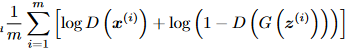
For each index i in the dataset, x^{(i)} is a real image from the dataset, and G(z^{(i)}) is an image generated by the generator from a noise vector z^{(i)}. Remember that we want to maximize this function: this entails maximizing log(D(x^{(i)})) (i.e. classify real images as real) and minimizing D(G(z^{(i)})) (i.e. classify fake images as fake). We implement this loss as follows:
1
2
3
4
5
6
7
8
9
10
11
12
13
14
15
16
17
18
19
20
impl GenerativeAdverserial {
    ...
    // The loss of the discriminator on some input batch composed of real and generated samples
    // the first batch_size samples are real, while the rest are counterfeit
    fn disc_loss(net_out: &Array2<f64>) -> f64 {
        let m = net_out.nrows() / 2;
        let real_range: Vec<usize> = (0..m).collect();
        let fake_range: Vec<usize> = (m..2*m).collect();
        let real_samples = net_out.select(Axis(0), &real_range);
        let fake_samples = net_out.select(Axis(0), &fake_range);

        // We take the sum of the logs of the predicted probabilties of each real sample
        // plus the sum of the logs of the complement of the predicted probabilities for each fake sample
        let loss = real_samples.map(|x| x.log2()).sum() +
               fake_samples.map(|x| (1f64 - x).log2()).sum();

        (1f64 / m as f64) * loss
    }
    ...
}
As written in the comments, to compute the loss, we pass the function the output of the network on a batch composed of m real images, and m fake images. The real images are images 0 through m-1, and the fake images are images m through 2m-1.
The generator’s loss is defined as follows (also taken from the GAN paper, algorithm 1):
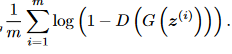
We want to minimize this function, which is done by maximizing D(G(z^{(i)})) (i.e. making the discriminator classify fake images as real). In practice, this function isn’t actually used when training the generator, because it has a problem which we can see if we plot the graph of log(1 - x):
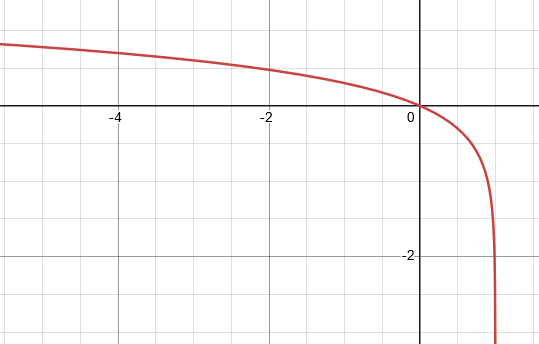
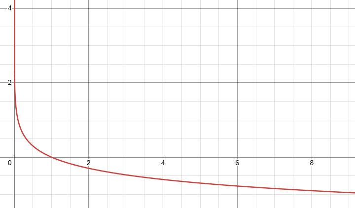
The gradient of the function is fairly low for low values of x, which means that GD will take a long time to converge. To fix this problem, we change the generator’s loss to the following function, which has an equivalent meaning (make the discriminator classify fake images as real):

The graph of -log(x) has a better slope indeed has better slope, so GD will converge faster:
We train the two networks alternatingly: the discriminator is trained for one batch, and then the generator is trained for one batch. This makes the training process a bit unstable, and there exist other variants of GANs that try to make the process more stable.
Once we’ve trained both models up to a sufficient point, we discard the discriminator, and then only use the generator to generate fake images given noise vectors. Here’s the code for the training process (I’ve only included the code for the training itself; in the real code there’s also a part that saves the intermediate images to a directory):
1
2
3
4
5
6
7
8
9
10
11
12
13
14
15
16
17
18
19
20
21
22
23
24
25
26
27
28
29
30
31
32
33
34
35
36
37
38
39
40
41
42
43
44
45
46
47
48
49
50
51
52
53
54
55
56
57
58
59
60
61
62
63
64
65
66
67
68
69
70
71
    pub fn fit(&mut self, x: Array2<f64>) {
        // Extract training hyperparameters
        let num_epochs = self.discriminator.num_epochs();
        let learning_rate = self.discriminator.learning_rate();
        let batch_size = self.discriminator.batch_size();
        let disc = &mut self.discriminator;
        let gen = &mut self.generator;
        let batches_per_epoch = x.nrows() / batch_size;

        for num_epoch in 0..num_epochs {
            for _ in 0..batches_per_epoch {
                // Begin discriminator training step
                // Sample minibatch of m training samples
                let mut input_batch = x.random_sample(batch_size);
                // Sample minibatch of m noise vectors, each of NOISE_DIM dimensions
                let noise_batch = Array2::noise_sample(batch_size, NOISE_DIM);
                let gen_samples = gen.forward(&noise_batch.view(), false);
                // Concatente them into one matrix, since we want the discriminator
                // to run both on the input and on the noise and produce probabilities for each sample
                input_batch.append(Axis(0), gen_samples.view()).unwrap();
                // Run the discriminator
                disc.forward(&input_batch.view(), true);
                // Get the gradients by running the backward pass
                let net_out = &disc.cache_last();
                let dy = GenerativeAdverserial::upstream_disc(net_out);
                let mut gradients = disc.backward(dy).0;
                gradients.reverse();
                // Perform a GD step on the discriminator
                for i in 0..disc.layers.len() {
                    // The current gradient
                    let grad = &gradients[i];

                    // Proceed only if there are parameter gradients
                    // layers such as ReLU don't have any parameters, so we don't need to update anything
                    if let (Some(dw), Some(db)) = grad {
                        disc.layers[i].update_params(&dw, &db, learning_rate);
                    }
                }
                // End discriminator training step
                // Begin generator training step
                // Sample minibatch of m noise vectors, each of NOISE_DIM dimensions
                let noise_batch = Array2::noise_sample(batch_size, NOISE_DIM);
                // Run the generator on the noise to generate new samples mimicing the training data
                let gen_samples = gen.forward(&noise_batch.view(), true);
                // Run the discriminator on the generated samples
                disc.forward(&gen_samples.view(), true);
                // The output of the discriminator on the generated images
                let disc_out = disc.cache_last().clone();
                // The first element in the discriminator's cache (the gradient of the discriminator)
                // WRT the generated samples
                // is used to compute the gradient of the generator
                let dy = GenerativeAdverserial::upstream_disc(&disc_out);
                let gen_grads = disc.backward(dy).1;
                // Get the gradient by running the backward pass
                let dy = GenerativeAdverserial::upstream_gen(&gen_samples, &disc_out, &gen_grads);
                let mut gradients = gen.backward(dy).0;
                gradients.reverse();
                // Perform a GD step on the generator
                for i in 0..gen.layers.len() {
                    // The current gradient
                    let grad = &gradients[i];

                    // Proceed only if there are parameter gradients
                    // layers such as ReLU don't have any parameters, so we don't need to update anything
                    if let (Some(dw), Some(db)) = grad {
                        gen.layers[i].update_params(&dw, &db, learning_rate);
                    }
                }
            }
        }
    }
The code starts by sampling a random set of rows from the input data x. Then, it creates a batch_size by noise_dimension matrix, where each row is a noise vector sampled from a Gaussian distribution. It then calls the generator on each row of this matrix to generate fake images. After this, it concatenates the real images sampled from the dataset with the fake images generated by the generator into one matrix input_batch. Afterwards, it runs the discriminator on this input batch to save the outputs of the hidden layers, which it uses to perform backprop, and then GD. To compute the upstream gradient dy (i.e. the gradient of the loss function WRT the output of the discriminator), it uses the function upstream_disc, which I’ll explain shortly. To train the generator, we start by sampling a matrix of random noise vectors, and call the generator on them to generate fake images. Then, we run the discriminator in training mode on those fake images, and save the output of the discriminator to disc_out. We then run the backward pass on the discriminator, which gives us the gradient of the discriminator’s loss WRT the fake images (this is useful later when performing backprop on the generator). Finally, we compute the the gradient of the generator’s loss WRT the fake images (i.e. the output of the generator) using the upstream_gen function, and then run the backward pass of the generator, which is used to perform GD. Now, let’s go through the upstream_desc and upstream_gen functions. As mentioned before, these functions are responsible for computing the gradient of the discriminator/generator’s loss function function WRT the discriminator/generator’s output: For example, upstream_desc computes the gradient of L, the discriminator’s loss, WRT D(x^{(i)}) and D(G(z^{(i)})) for all i. We derive the upstream gradient of the discriminator as follows:
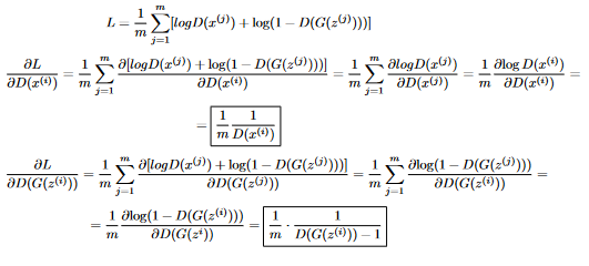
We split the task into two parts: deriving L WRT D(x^{(i)}) (real images) and deriving L WRT D(G(z^{(i)})) (fake images). In both cases the approach is the same: we first get rid of the sum, since the value of D(x^{(i)}) doesn’t impact any other component of the sum. Then, we’re left with two pretty simple derivatives: the derivative of log(x) and the derivative of log(1 - x) and we get our result. In the code, we implement this as follows:
1
2
3
4
5
6
7
8
9
10
11
12
13
14
15
16
17
18
19
20
21
22
23
24
25
26
27
    // The upstream gradient of the Discriminator's loss WRT the discriminator's output on
    // a batch containing generated samples and real samples
    fn upstream_disc(net_out: &Array2<f64>) -> Array2<f64> {
        // The first half of the outputs are probabilities for real training samples
        // The other half are probabilities for samples generated from noise by the generator
        let m = net_out.nrows() / 2;
        let mut out_grad = Array2::zeros((0, 1));

        // The upper half
        for i in 0..m {
            let prob_xi = net_out.row(i)[0];
            // Derivative of log(D(x_i)) WRT D(x_i) is 1 / D(x_i)
            let dprob_xi = 1f64 / prob_xi;
            let to_push = Array1::from_elem(1, dprob_xi);
            out_grad.push_row(to_push.view()).unwrap();
        }
        // The lower half
        for i in m..2 * m {
            let prob_gzi = net_out.row(i)[0];
            // Derivative of log(1 - D(G(z_i))) WRT D(G(z_i)) is 1 / (D(G(z_i)) - 1)
            let dprob_gzi = 1f64 / (prob_gzi - 1f64);
            let to_push = Array1::from_elem(1, dprob_gzi);
            out_grad.push_row(to_push.view()).unwrap();
        }

        -1f64 * (1f64 / m as f64) * out_grad
    }
In the end, we multiply by -1, since even though we’re looking to maximize this function, the code only does gradient descent, so instead we’ll resort to minimizing the negative of the function. Now, let’s derive the upstream gradient for the generator:
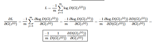
Like earlier, we start with getting rid of the sum, and then we use the chain rule to get rid of the log. We’re left with the constant -1/m, 1 / D(G(z^{(i)})), and the derivative of D WRT G(z^{(i)}). This is why, earlier, when training the generator, we also needed to run the backward pass for the discriminator:
1
2
3
4
5
6
7
8
9
10
11
12
13
14
// Begin generator training step
// Sample minibatch of m noise vectors, each of NOISE_DIM dimensions
let noise_batch = Array2::noise_sample(batch_size, NOISE_DIM);
// Run the generator on the noise to generate new samples mimicing the training data
let gen_samples = gen.forward(&noise_batch.view(), true);
// Run the discriminator on the generated samples
disc.forward(&gen_samples.view(), true);
// The output of the discriminator on the generated images
let disc_out = disc.cache_last().clone();
 // The first element in the discriminator's cache (the gradient of the discriminator)
// WRT the generated samples
// is used to compute the gradient of the generator
let dy = GenerativeAdverserial::upstream_disc(&disc_out);
let gen_grads = disc.backward(dy).1;
The gen_grads variable contains the gradient of the discriminator WRT its input, which in our case are the fake images. In other words, gen_grads contains

Which is exactly what we need! Here’s the implementation for computing the upstream gradient of the generator:
1
2
3
4
5
6
7
8
9
10
11
12
13
14
15
16
17
18
19
20
21
22
23
24
25
26
    // The gradient of the Generator's loss WRT each pixel in each image
    // in the generator's batch
    fn upstream_gen(
        net_out: &Array2<f64>,
        disc_out: &Array2<f64>,
        dy_dgzi: &Array2<f64>,
    ) -> Array2<f64> {
        // net_out contains the generated images, of shape (batch_size, img_size)
        let m = net_out.nrows();
        // The gradient of the loss WRT each pixel in each output image
        // shape: (batch_size, img_size)
        let mut out_grad = Array2::zeros((0, IMAGE_SIZE*IMAGE_SIZE));

        // Compute the gradients
        for i in 0..m {
            let prob_gzi = disc_out.row(i)[0];
            // Derivative of log(D(G(z_i))) WRT D((G(z_i))) is 1 / D(G(z_i)))
            let dprob_gzi = 1f64 / prob_gzi;
            // The gradient of the loss WRT counterfeit i
            let dy_curr = dy_dgzi.row(i);
            let to_push = dy_curr.map(|x| x * dprob_gzi);
            out_grad.push_row(to_push.view()).unwrap();
        }

        (1f64 / m as f64) * out_grad
    }
The Results
Awesome! Now we have everything we need to create GANs, which can produce cool animations like the following one:
The above GIF shows a GAN whose discriminator has layers of the form 784x500x500x1, and whose generator has layers of the form 100x500x500x784 training for 30 epochs to generate an image of the digit 7 (it’s trained on all instances of a 7 from MNIST). The batch size is set to 64 and the learning rate is set to 0.003. Here’s the code to do that:
1
2
3
4
5
6
7
8
9
10
11
12
13
14
15
16
17
18
19
20
21
22
fn main() {
    let args = Args::parse();
    let dataset = parse_dataset(&args.mnist_path);

    let mut gan = GenerativeAdverserial::new(50, 64, 0.003, Some(args.inter_path));
    // Our discriminator
    gan.discriminator.add_layer(Box::new(Linear::new(784, 500)));
    gan.discriminator.add_layer(Box::new(ReLU::new()));
    gan.discriminator.add_layer(Box::new(Linear::new(500, 500)));
    gan.discriminator.add_layer(Box::new(ReLU::new()));
    gan.discriminator.add_layer(Box::new(Linear::new(500, 1)));
    gan.discriminator.add_layer(Box::new(Sigmoid::new()));
    // Our generator
    gan.generator.add_layer(Box::new(Linear::new(100, 500)));
    gan.generator.add_layer(Box::new(ReLU::new()));
    gan.generator.add_layer(Box::new(Linear::new(500, 500)));
    gan.generator.add_layer(Box::new(ReLU::new()));
    gan.generator.add_layer(Box::new(Linear::new(500, 784)));
    gan.generator.add_layer(Box::new(Sigmoid::new()));
    // Train it
    gan.fit(dataset.data);
}
The args.inter_path variable just tells the program where to save the images. Let’s plot the losses of the generator and the discriminator:
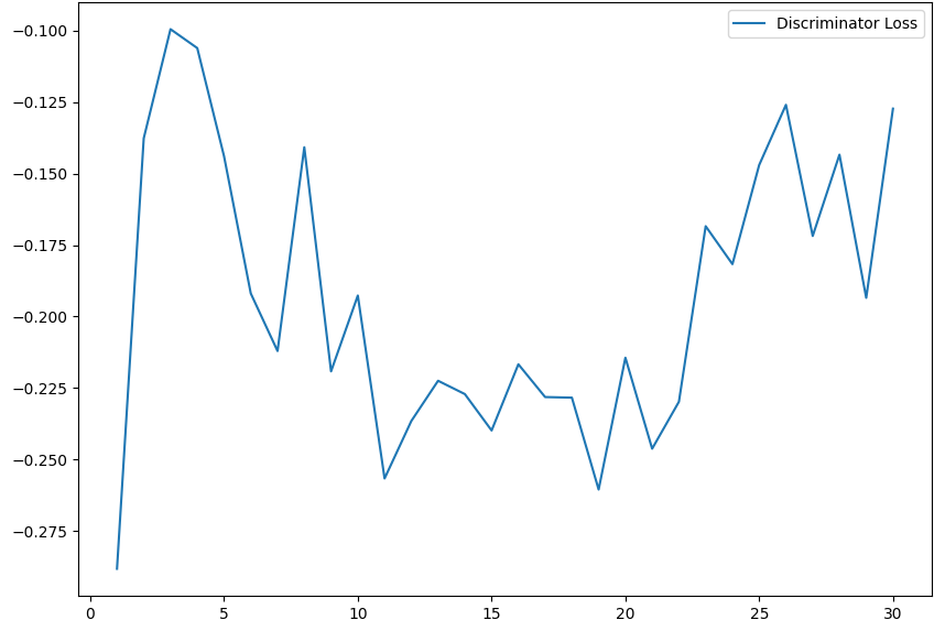
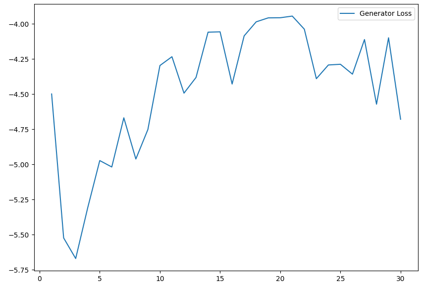
As we can see, the training isn’t very stable; this is probably caused by the fact that we train the models in an alternating fashion. Nonetheless, the images we managed to get look like real 7s, which I find very cool!
What’s Next
There are two main things I want to improve in this implementation:
- Change the
backwardfunctions to allow for more types of layers, since currently the signature is:
1
2
3
4
5
	    fn backward(
        &self,
        dy: Array2<f64>,
        x: Array2<f64>,
    ) -> (Array2<f64>, Option<Array2<f64>>, Option<Array1<f64>>);
Which only allows us to return the gradients WRT the input, a matrix, and a vector. Changing this allows us to implement more complex GANs, such as DCGANs (Deep Convolutional GANs), which include convolutional layers, and hence generate more complex images
- Introduce CUDA support to allow training the model on the GPU - this lets the model train for far more epochs much quicker, and besides it seems like a very interesting topic :) Thanks for reading! I had a lot of fun putting this post together, and I hope you learned from it as much as I did :) Yoray P.S. All the code for the post can be found in this repo