Digit Recognition with Rust and WASM - Part 1

Prelude

Hello Everyone! This post is the first in a two-part series where we implement a WebApp that recognizes digits from scratch:

• In this part, we implement a Neural Network from scratch in Rust. The math behind Neural Networks (or Neural Nets for short) is explained here, so you don’t have to know anything about them to read this post :)
• In the second part, we construct a frontend that interacts with the Rust backend using WASM (WebAssembly) Prerequisites: Some knowledge of Linear Algebra (Matrices, Vectors) and Multivariable Calculus (Partial Derivatives, Gradients, The chain rule) is recommended

  Digit Recognition

  In this post we tackle the problem the problem of digit recognition, which is considered the “Hello World” of machine learning: Given some 28x28 grayscale image, we need to determine what digit it represents (examples of inputs with their corresponding digits are presented in the next figure). This type of problem is called multiclass classification, because we need to classify each image into exactly one of 10 classes. 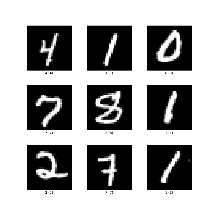1 Source: https://www.researchgate.net/figure/Example-images-from-the-MNIST-dataset_fig1_306056875 To help us, we are provided a dataset (MNIST) of 70000 handwritten digits together with what digit they represent (this is called the label, and it’s what we’re trying to predict). This dataset is provided in a CSV file, and we parse it with the following code:

const NUM_FEATURES: usize = 784;
const LINE_SIZE: usize = 785;
const NUM_CLASSES: usize = 10;
const GREYSCALE_SIZE: f64 = 255f64;

/// Represents the dataset 
struct Dataset {
    data: Array2<f64>,
    target: Array2<f64>, // Target labels in one-hot encoding
}

/// Parse a record (e.g. CSV record) of the form <x1><sep><x2><sep>...
/// Returns a vector of the xi's if the function was succesful
/// and None otherwise
fn parse_line<T: FromStr>(s: &str, seperator: char) -> Option<Vec<T>> {
    let mut record = Vec::<T>::new();

    for x in s.split(seperator) {
        match T::from_str(x) {
            Ok(val) => {
                record.push(val);
            }
            _ => return None,
        }
    }

    Some(record)
}

/// Parse a line in the dataset. Return the pixels and the label
/// Line is stored in the format: <label>,<pixel0x0>,<pixel0x1>,...
/// The dataset is taken from here https://www.kaggle.com/datasets/oddrationale/mnist-in-csv
fn parse_dataset_line(line: &str) -> Option<(Vec<f64>, f64)> {
    match parse_line(line, ',') {
        Some(v) => match v.len() {
            // we divide by 255 to normalize
            LINE_SIZE => Some((
                v[1..LINE_SIZE].iter().map(|x| x / GREYSCALE_SIZE).collect(),
                v[0],
            )),
            _ => None,
        },
        _ => None,
    }
}

// Return matrix that represents the dataset
fn parse_dataset(path: &str) -> Dataset {
    let file = File::open(path);
    let mut data = Array::zeros((0, NUM_FEATURES));
    let mut target = Array::zeros((0, NUM_CLASSES));
    let mut contents = String::new();

    file.unwrap().read_to_string(&mut contents).unwrap();

    for line in contents.lines().skip(1).take_while(|x| !x.is_empty()) {
        let line = parse_dataset_line(line).unwrap();
        let pixels = line.0;
        let label = line.1 as usize;
        // Construct one-hot encoding for the label
        let one_hot_target: Vec<f64> = (0..NUM_CLASSES)
            .map(|idx| if idx == label { 1f64 } else { 0f64 })
            .collect();

        data.push_row(ArrayView::from(&pixels)).unwrap();
        target.push_row(ArrayView::from(&one_hot_target)).unwrap();
    }

    Dataset { data, target }
}

Now that we parsed the dataset, we can use it to train the neural net.

Neural Networks

Note: Throughout this post I use the term “Neural Networks” to refer to feedforward, fully connected neural networks, although there exist other types of neural nets like Convolutional Neural Networks and Recurrent Neural Networks Neural Networks (invented in 1943 by Warren McCulloch and Walter Pitts) are one of the most fundamental and popular models in the field of Machine Learning. They are inspired by the brain, and are composed of layers of varying sizes. Each layer is composed of units called neurons.

• The first layer in the network is called the input layer, and as you probably guessed, gets the input of the problem. It is composed of special neurons called passthrough neurons that output whatever their input is. In our case, the input layer consists of 28x28=784 passthrough neurons. Each one represents a greyscale pixel, and gets a value in the range 0-1 (because we normalized the pixels when parsing the dataset).
• The last layer in the network is called the output layer, and outputs the output of the problem. It’s size varies based on the problem. In the case of digit recognition, it consists of 10 neurons, with neuron i representing the score for how sure the network is of the input being the digit i. Because digit recognition is a multiclass classification problem, we also apply the softmax function to the outputs of the output layer to convert the scores to a probability distribution. The code for the softmax function is:

/// Softmax function - Convert scores into a probability distribution
fn softmax(scores: ArrayView1<f64>) -> Array1<f64> {
    let max = scores.iter().max_by(|x, y| x.total_cmp(y)).unwrap();
    // We use a numerical trick where we shift the elements by the max, because otherwise
    // We would have to compute the exp of very large values which wraps to NaN
    let shift_scores = scores.map(|x| x - max);
    let sum: f64 = shift_scores.iter().map(|x| x.exp()).sum();

    (0..scores.len())
        .map(|x| shift_scores[x].exp() / sum)
        .collect()
}

• All other layers lie between the input and the output layer, and are called hidden layers. They can be of any size, but different sizes and number of hidden layers will of course affect the performance of the network. Each neuron i in layer k is connected to every neuron j in layer k+1 with some weight w^k_{i, j}. There is also a special neuron in every layer (except for the output layer) called the bias neuron. The bias neuron always outputs 1, and is also connected to every neuron in the next layer. Throughout this post, we denote the weight between the bias neuron in layer k with neuron i in layer k+1 with b^k_i. Now let’s go through what each individual neuron does:
• The neurons in the input layer are called passthrough neurons, and output whatever their input is.
• The output of neuron j in layer k, where k is neither the first layer nor the last layer is 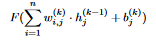where F is some nonlinear activation function. The activation function is used to introduce nonlinearity into the network, because otherwise the network could only solve simple, linear problems. The other part (the input of F) means multiplying each of the outputs of the neurons in the previous layer (layer k-1) with the weights connecting them to neuron j in layer k. We add the term b^k_j because the value of the bias neuron is always 1
• The output of each neuron j in the output layer is 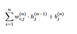This is the same as in the hidden layers, but without applying the activation function (because the output layer represents the output to the problem, so applying the activation function on it makes no sense) Common activation functions include:
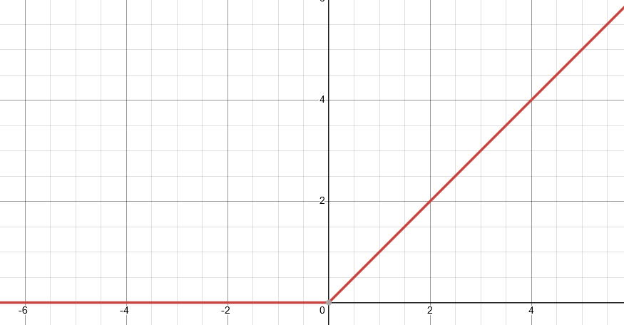
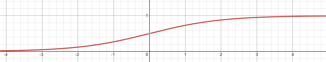
• ReLU (Rectified Linear Unit): $ReLU(z) = max(0, z)$ 2
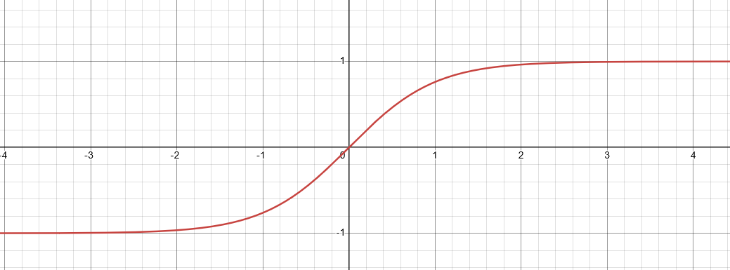
• Sigmoid: $\sigma(z) = \frac{1}{1 + e^{-z}}$ 3
• Hyperbolic Tangent: $\tanh(z)$ 4 Let’s do an example of computing the values of each of the neurons in the following network: 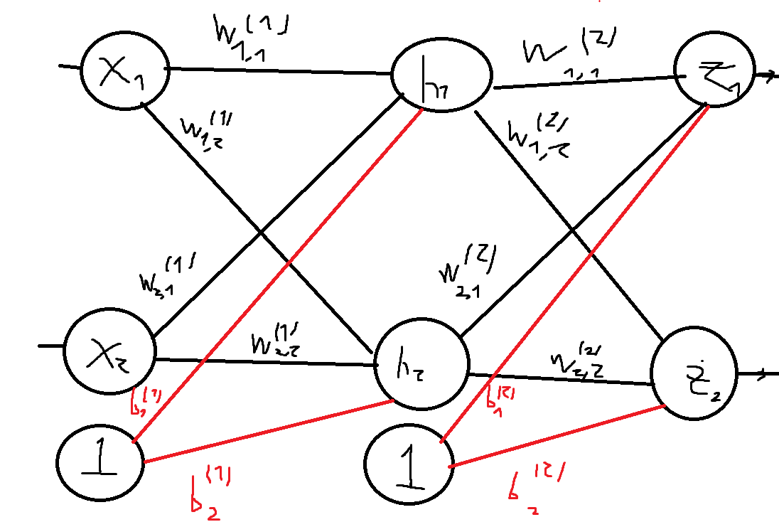4 The outputs of neurons h1 and h2 are: 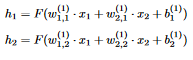5 Where F is the activation function And the outputs of the neurons z1 and z2 in the output layer are: 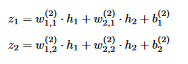6 Note that the output of layer k (except for the last layer, where the output is the same but we don’t apply the activation function), expressed with matrix multiplications is: 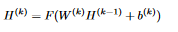7 In words, this means that the output of layer k is the weight matrix between layer k-1 and layer k dot the output of layer k-1 plus the bias between layer k-1 and layer k. If W^k dot H^(k-1) contains multiple rows, the addition of the bias vector is broadcasted by adding it to every row of the matrix. This happens when multiple instances are inputted to the network. Note that if we input multiple instances to the network at the same time (we do this by adding a row for each instance in the input matrix), each neuron outputs a column vector and not a number like when the input matrix contains one row. We can use this to implement the forward pass of the network, which means computing the values of each of the layers (throughout this project we use the ReLU function as the activation function):

/// Represents a neural net
struct NeuralNet {
    layers: Vec<(Array2<f64>, Array1<f64>)>, // Each layer holds a weight matrix and a bias vector
    num_epochs: usize,                       // Training hyperparams
    batch_size: usize,
    learning_rate: f64,
}

impl NeuralNet {
    /// Construct a new neural net according to the specified hyperparams
    pub fn new(
        layer_structure: Vec<usize>,
        num_epochs: usize,
        batch_size: usize,
        learning_rate: f64,
    ) -> NeuralNet {
        let mut layers = vec![];
        let mut rng = rand::thread_rng();
        // Weights are initialized from a uniform distribiution
        let distribution = Uniform::new(-0.3, 0.3);

        for i in 0..layer_structure.len() - 1 {
            // Random matrix of the weights between this layer and the next layer
            let weights = Array::zeros((layer_structure[i], layer_structure[i + 1]))
                .map(|_: &f64| distribution.sample(&mut rng));
            // Bias vector between this layer and the next layer. Init'd to ondes
            let bias = Array::ones(layer_structure[i + 1]);

            layers.push((weights, bias));
        }

        NeuralNet {
            layers,
            num_epochs,
            batch_size,
            learning_rate,
        }
    }

    // Perform a forward pass of the network on some input.
    // Returns the outputs of the hidden layers, and the non-activated outputs of the hidden layers (used for backprop)
    fn forward(&self, inputs: &ArrayView2<f64>) -> (Vec<Array2<f64>>, Vec<Array2<f64>>) {
        let mut hidden = vec![];
        let mut hidden_linear = vec![];
        // The first layer is a passthrough layer, so it outputs whatever its input is
        hidden.push(inputs.to_owned());

        // We iterate for every layer
        let mut it = self.layers.iter().peekable();

        // Iterate over the layers
        while let Some(layer) = it.next() {
            // The output of the layer without applying the activation function
            let lin_output = hidden.last().unwrap().dot(&layer.0) + &layer.1;
            // The real output of the layer - If the layer is a hidden layer, we apply the activation function
            // and otherwise (this is the output layer) the output is the same as the linear output
            let real_output = lin_output.map(|x| match it.peek() {
                Some(_) => relu(*x),
                None => *x,
            });

            hidden.push(real_output);
            hidden_linear.push(lin_output);
 
        }

        (hidden, hidden_linear)
    }


    /// Predict the probabities for a set of instances - each instance is a row in "inputs"
    fn predict(&self, inputs: &ArrayView2<f64>) -> Array2<f64> {
        let (hidden, _) = self.forward(inputs);
        let scores = hidden.last().unwrap();
        // Construct the softmax
        let mut predictions = Array::zeros((0, scores.ncols()));

        for row in scores.axis_iter(Axis(0)) {
            predictions.push_row(softmax(row).view()).unwrap();
        }

        predictions
    }
}

/// Activation function
fn relu(z: f64) -> f64 {
    z.max(0f64)
}

Now that we know what a Neural Net is, let’s see how to train it on the problem of Digit Recognition. Training is the process of tweaking the weights and biases until we get to a point where the network can classify

Training the Network

To train the network, we first need a measure of how bad the network did on a specific batch of inputs. This measure is called the loss function, and in the case of multiclass classification, the most common loss function is called the cross-entropy loss function, and is defined on some batch as 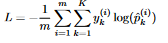8 , where:

• m is the number of inputs in the batch
• K is the number of classes (in our case 10)
• y^i_k is 1 if instance i is in class k and 0 otherwise,
• p^i_k is the probability that the network predicted of the i-th instance being in class k (the k-th value in the softmax result of instance i). This function is implemented as follows (actual is the network’s predictions and target is the target):

/// Calculate the cross-entropy loss on a given batch
fn cross_entropy(actual: &Array2<f64>, target: ArrayView2<f64>) -> f64 {
    let total: f64 = actual
        .axis_iter(Axis(0))
        .zip(target.axis_iter(Axis(0)))
        .map(|(actual_row, target_row)| target_row.dot(&actual_row.map(|x| x.log2())))
        .sum();

    -1f64 * (1f64 / actual.nrows() as f64) * total
}

To make the network perform well on the task of digit classification, we of course want to minimize this loss function. But how do we do that? This function is dependent on thousands of parameters (the weights and biases) and is super complicated, so we can’t just find its minimum like a “simple” function (finding where the derivative is zero, solving an equation etc.). If so, we’ll have to turn to other means, namely numerical approximations. The method we’ll use here is one of the most popular ones for approximating the minimum of a function, and is called Gradient Descent. It uses the property of the gradient that says that the gradient is the direction of steepest ascent, and conversely the direction opposite the gradient is the direction of steepest descent. A good analogy for this is to think of a ball standing somewhere on a curve. The ball always rolls in the steepest direction, until it gets to a point where the gradient is 0 (a minimum). The process is defined as follows:

1. Let \theta^1 be some random vector of length n.
2. Do 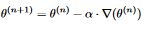Until you get to the desired accuracy The parameter $\alpha$ is called the learning rate, and determines the size of the steps we take. If we set it too high, the algorithm will diverge and not find a minimum. If we set it too low, we will take very small steps and possibly get stuck in a local minimum (where the gradient is 0, so standard GD can’t escape it). Here is an illustration on the function f(x, y) = x^2 + y^2: 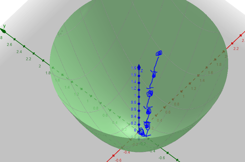9 Several variations of GD exist, such as Stochastic GD and mini-batch GD. Specifically, in this post, we use mini-batch GD, which is similar to standard GD, except that we take small batches (for example 50 instances) of the data each time and compute the gradient of the loss function with respect to the batch, and not WRT the entire dataset. We use this variation because it allows us to escape local minima, and is also faster. The code for training (“fitting”) the model to the dataset is shown here:

	    /// Fit the model to the dataset
    fn fit(&mut self, dataset: &Dataset, debug_path: &Option<String>) -> Option<Vec<(usize, f64)>> {
        // Used for writing the debug output
        let mut batch_cnt: usize = 0;
        let mut losses = vec![];
        let is_debug = !debug_path.is_none();

        for _ in 0..self.num_epochs {
            // Get a batch of instances and their targets
            for (input_batch, target_batch) in dataset
                .data
                .axis_chunks_iter(Axis(0), self.batch_size)
                .zip(dataset.target.axis_chunks_iter(Axis(0), self.batch_size))
            {
                let (hidden, hidden_linear) = self.forward(&input_batch);

                let scores = hidden.last().unwrap();
                let mut predictions = Array::zeros((0, scores.ncols()));

                // Construct softmax matrix
                for row in scores.axis_iter(Axis(0)) {
                    predictions.push_row(softmax(row).view()).unwrap();
                }

                // Push to the losses vector if we're in debug mode
                if is_debug {
                    let loss = cross_entropy(&predictions, target_batch);
                    losses.push((batch_cnt, loss));

                    batch_cnt += 1;
                }

                // Gradient is initialized to the gradient of the loss WRT the output layer
                let grad = predictions - target_batch;

                self.backward_and_update(hidden, hidden_linear, grad);
            }
        }

        match debug_path {
            Some(_) => Some(losses),
            None => None,
        }
    }

The backward_and_update function computes the gradients and performs the GD step; it uses an algorithm called Backpropagation (or Backprop for short) and is explained in the next section.

Backpropagation

Let’s do a little recap: We’ve defined what a neural net is, and defined a loss function that measures how bad the network did on a specific batch of images. Then, we saw how to minimize the loss function using Gradient Descent. If so, the only thing we have left is how to compute the gradients! Our goal is to compute the gradient of the loss function WRT every weight and bias in the network, to know how much to tweak each of them when performing the GD step (Computing the gradient WRT the inputs doesn’t make sense). To accomplish this, we use a process called Backpropagation (or backprop for short). The idea is to first compute the gradient WRT the neurons and weights in the last layer, and then propagate this gradient backward, one layer at a time using the chain rule. To illustrate how this is done, consider the next network: 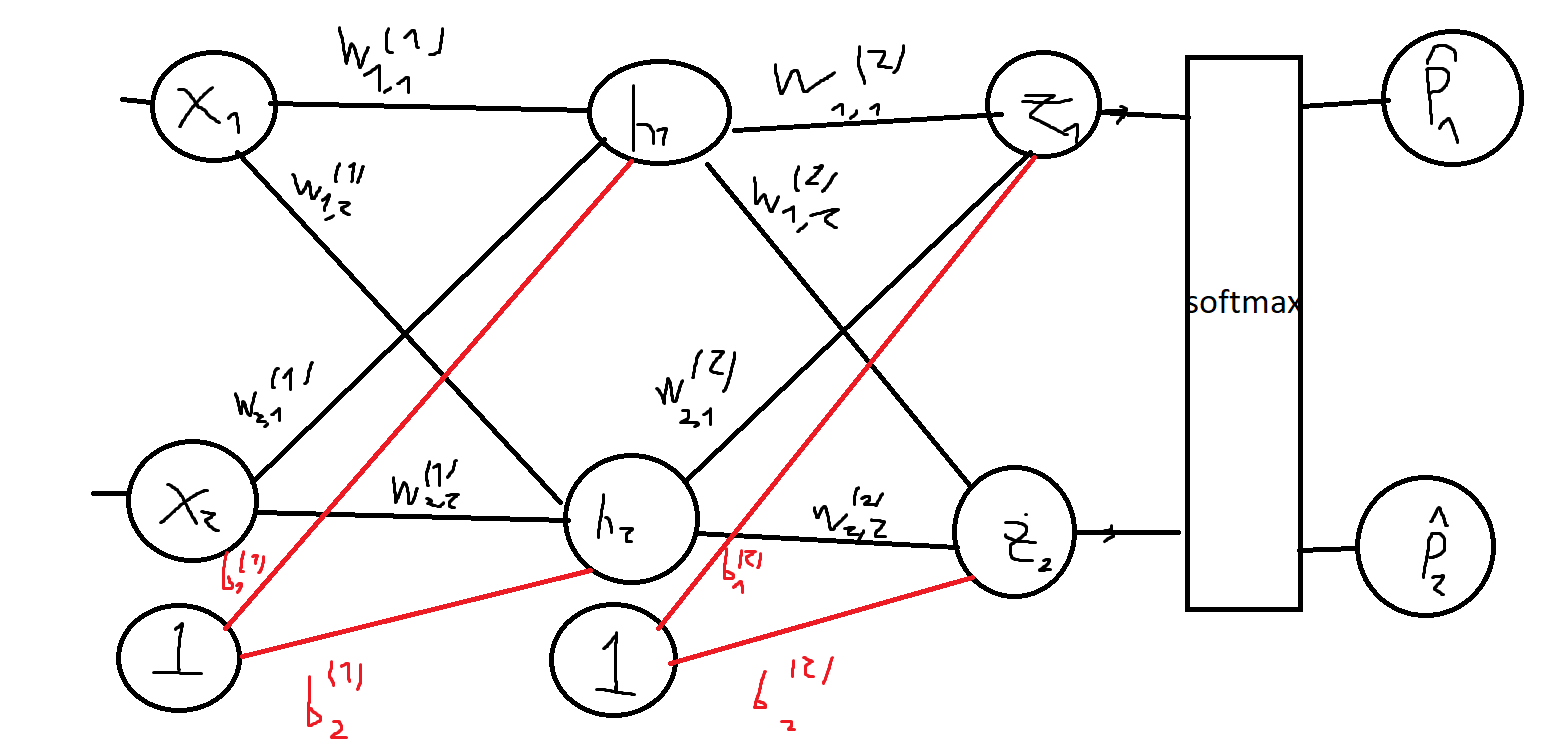10 Consider some input batch X with targets Y (The rows are one-hot encoded; row i is all zeroes except for entry k which is 1, where k is the class that instance i belongs to). Let the predictions of the network be P (Row i is the probability distribution that the network computed for instance i in X). Throughout this process, we use the fact that the partial derivative of L WRT z_i (neuron i in the output layer) is P_i -Y_i, where P_i is the i-th column of P, and Y_i is the i-th column of Y (I don’t show a proof for this here because this is not a super hard derivative to calculate and it’s not really the point) We start with computing the gradient of the loss function WRT the weights in the second layer. The chain rule tells us that 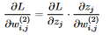11 Since the output of each neuron in the output layer is 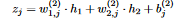12 the partial derivative of z_j WRT weight i,j in the output layer is easy to calculate: 13 Note that since X contains multiple instances, each h_i is a column vector and not a number. The other derivative (The loss function WRT z_j) comes out to be P_j - Y_j from what we’ve mentioned earlier, and so 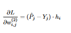14 We can also express this with matrix multiplication (this will come in handy later when we implement the algorithm): 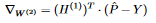15 Similarily, for the biases, we have 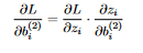16 The right derivative (z_j WRT the bias) comes out to be 1, and so 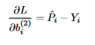17 This is a matrix with multiple rows, while the bias vector is only a vector, so we take the mean over all the rows. Now let’s move on to the weights and biases in layer 1. As before, we get 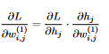18 This time there are two differences from the previous calculation:

1. The neurons in the hidden layer apply the activation function, while the neurons in the output layer do not
2. The neurons in the hidden layer impact both z_1 and z_2, which in turn impact the loss function We start with the right derivative (the output of the neuron WRT the weight). The output of neuron h_j is 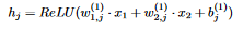19 This is just a composition of functions, so we can use the chain rule! Let 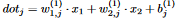20 (This is why we saved the non-activated outputs of the layers when we did the forward pass). We have h_j = ReLU(dot_j), and so 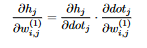21 The derivative of ReLU is the step function: step(x) = (x > 0) ? 1 : 0. Mathematically, it is undefined at x=0, but in practice we set it to 0. If so, 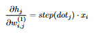22 Now we compute the other derivative (the loss function WRT h_j). As we mentioned earlier, h_j affects both the value of z_1 and the value of z_2, which, in turn, affect the loss function: 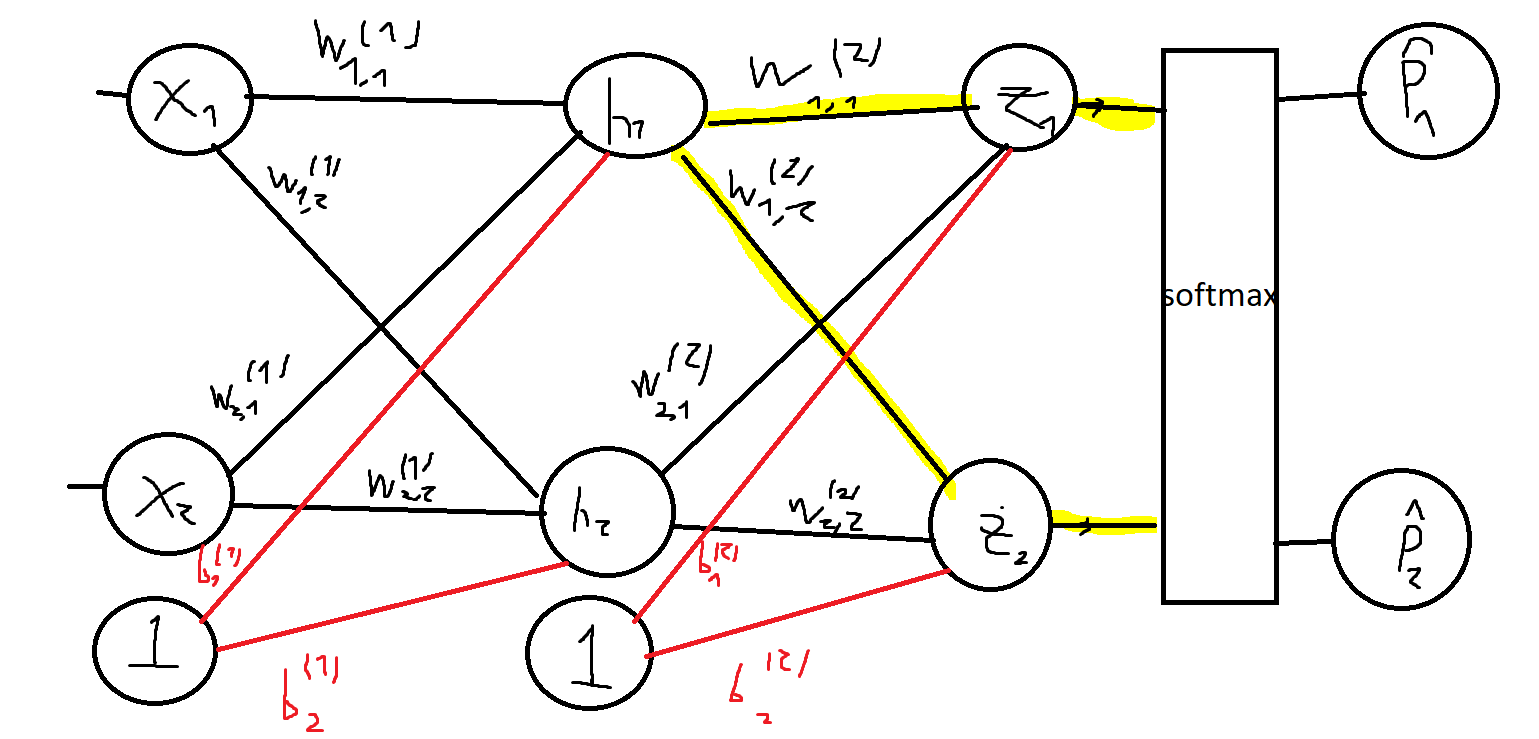23 To use the chain rule we add up the upper chain and the lower chain: 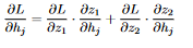24 This comes out to be 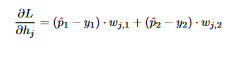25 We conclude that 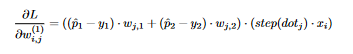26 In terms of matrix multiplication, we have 27 , where ⊙ means element-wise multiplication. The calculation for the gradients with respect to the biases is very similar, so I didn’t show it here :) The complete code for the backprop is:

        /// Calculate the gradients using backprop and perform a GD step
    fn backward_and_update(
        &mut self,
        hidden: Vec<Array2<f64>>,
        hidden_linear: Vec<Array2<f64>>,
        grad: Array2<f64>,
    ) {
        // The gradient WRT the current layer
        let mut grad_help = grad;

        for idx in (0..self.layers.len()).rev() {
            // If we aren't at the last layer, we need to change the gradient
            if idx != self.layers.len() - 1 {
                let step_mat = hidden_linear[idx].map(|x| step(*x));
                grad_help = grad_help * step_mat;
            }

            // Gradient WRT the weights in the current layer
            let weight_grad = hidden[idx].t().dot(&grad_help);
            // Gradient WRT the biases in the current layer
            let bias_grad = &grad_help.mean_axis(Axis(0)).unwrap();

            // Perform GD step
            let new_weights = &self.layers[idx].0 - self.learning_rate * weight_grad;
            let new_biases = &self.layers[idx].1 - self.learning_rate * bias_grad;

            // Update the helper variable
            grad_help = grad_help.dot(&self.layers[idx].0.t());

            self.layers[idx] = (new_weights, new_biases);
        }
    }

/// Derivative of ReLU
fn step(z: f64) -> f64 {
    if z >= 0f64 {
        1f64
    } else {
        0f64
    }
}

Summary

We’ve successfully built a Neural Network to solve the problem of digit recognition! In the complete project, which you can find here, I also added support for command line arguments (specifying the training hyperparameters and debug mode). Here is the graph of the loss function changing over training: 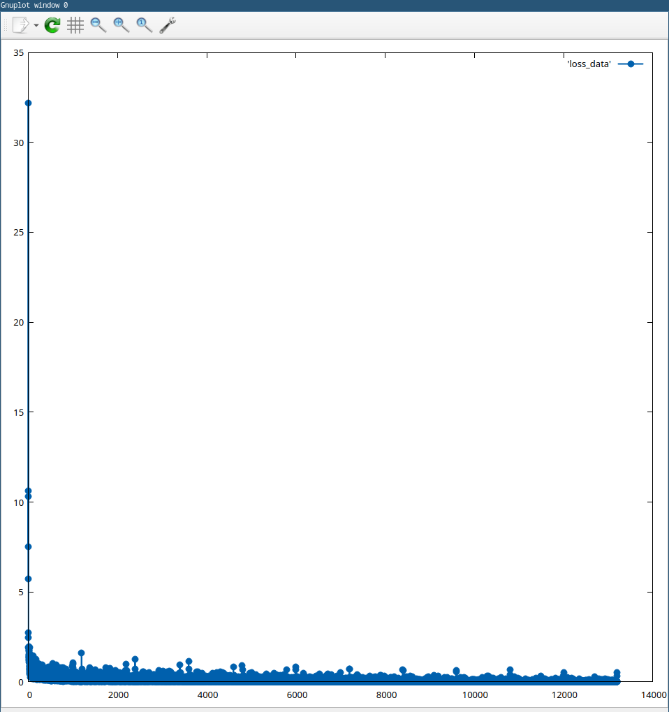28 We achieved a pretty good loss (270/10000 = 2.7% on the graph shown above), although this can be further improved, for example by doing early stopping or adding regularization, but I wanted to keep it simple for now. This was a really fun and difficult project to work on, and I’ve learned a lot both about ML and Rust. If you found any mistakes in the post, let me know :)

As always, thank you for reading❤️!!!!!!!!! Yoray